See the latest book content here.
5 Convolutional Neural Networks
Consider first this cute video:
In the video we see that “Chaser” the dog can recongize a thousand stuffed animals based on hearing their name. It requires him to recognize the spoken name, recognize the image, and make the associated connections. This type of thinking task is very topical for this unit where we’ll see how convolutions, mixed with artificial neural networks can be very powerful. They allow autonomous systems can be trained to classify images, and much more.
This resource by A. Amidi and S. Amidi provides a useful summary of some of the material that we cover here. Here is the interactive version.
We begin with some background about convolutions and then move onto neural networks to see how convolutions interpaly with neural networks.
5.1 Background on convolutions
A convolution can also be defined as an operation on two functions. This is often the case when considering continuous time convolutions as is done in electrical engineering, control theory, and the study of differential equations. However in our context, we mostly focus on vectors, matrices, and tensors. A convolution is an operation on two vectors, matrices, or tensors, that returns a third vector, matrix, or tensor.
5.1.1 Convolutions in LTI systems
LTI systems are concepts from control theory and signal processing that have influenced machine learning an led to the development of convolutional neural networks. To get a feel for the importance of convolutions lets first consider linear time invariant (LTI) systems where we focus on scalar valued, discrete time systems (e.g. \(t = \ldots,-2,-1,0,1,2,\ldots\)).
An LTI system, denoted \({\cal O}\Big(\cdot\Big)\), maps an input sequence to an output sequence (this is called a system), and has the following two properties:
Linearity: For input signals \(x_1(t)\) and \(x_2(t)\) and scalars \(\alpha_1\) and \(\alpha_2\), \[ {\cal O}\Big(\alpha_1 x_1(\cdot) + \alpha_2 x_2(\cdot) \Big)(t) = \alpha_1 {\cal O}\Big( x_1(\cdot)\Big)(t) + \alpha_2 {\cal O}\Big( x_2(\cdot) \Big)(t). \]
Time invariance: Assume the input signal \(x(\cdot)\) has output \(y(\cdot) = {\cal O}\Big(x(\cdot) \Big)\). Take now the time shifted input \(\tilde{x}(t) = x(t-\tau)\) then output of \({\cal O}\Big(\tilde{x}(t)\Big)\), denoted \(\tilde{y}(\cdot)\), is the time shifted output of the original input. Namely \(\tilde{y}(t) = y(t - \tau)\).
It turns out that many operations on signals are well described by LTI systems. Further, it turns out that the operation of any LTI system on an input signal is equivalent to a convolution of the input signal with a special signal associated with the system, denoted the impulse response. We describe both convolutions and the impulse response shortly.
Observe that \(\delta(t-\tau)\) is the time shifted version of \(\delta(t)\) and is \(1\) at \(t = \tau\) and \(0\) for any other \(t\). Consider any signal \(x(t)\). It can be represented as, \[ x(t) = \sum_{\tau = -\infty}^\infty x(\tau)\delta(t-\tau), \] where \(\delta(t)\) is the sequence such that \(\delta(0) = 1\) and for \(t \neq 0\), \(\delta(t) = 0\).
We can now use this representation together with the LTI properties: Here we used the linearity property since \(x(\tau)\) are constants with respect to the time variable \(t\). \[\begin{align*} y(t) &= {\cal O}\Big(x(t) \Big)\\ &= {\cal O}\Big(\sum_{\tau = -\infty}^\infty x(\tau)\delta(t-\tau) \Big) \\ &= \sum_{\tau = -\infty}^\infty x(\tau) {\cal O} \Big( \delta(t-\tau) \Big). \end{align*}\] Now denote the output of \(\delta(t)\) as \(h(t)\). This is called the impulse response. Then we due to time invariance \({\cal O}\Big( \delta(t-\tau) \Big) = h(t-\tau)\). We thus arrive at, \[ y(t) = \sum_{\tau = -\infty}^\infty x(\tau) h(t-\tau). \] Analogous results exist for continuous time systems, where the impulse response requires considering the generealized function, \(\delta(t)\), called the Dirac delta function. In that case the convolution \(x \star h\) is determined via, \[ \int_{\tau = -\infty}^\infty x(\tau)h(t-\tau) \, d\tau. \] This is called the convolution of \(x(\cdot)\) and \(h(\cdot)\) and is denoted \(y = x \star h\). Hence we see that convolutions arise naturally when considering linear time invariant systems because the operation of an LTI system on any signal is simply given via the convolution of the signal with the system’s impulse response.
This video illustrates the operation of a (discrete time) convolution operation. The common phrase is "flip, shift, and add’.
It is easy to see that the convolution operation is commutative. That is \(x \star h = h \star x\). Simply do this via a change of variables \(\tau' = t-\tau\) (or \(\tau = t- \tau'\)) \[ x \star h = \sum_{\tau = -\infty}^\infty x(\tau) h(t-\tau) = \sum_{\tau' = -\infty}^\infty x(t-\tau') h(\tau') = h \star x. \]
Now note that if we were to define the convolution operation differently (here denoted \(\tilde{\star}\)), as, \[ x \,\tilde{\star} \, h = \sum_{\tau = -\infty}^\infty x(\tau) h(\tau - t), \] then it no longer holds that \(x \,\tilde{\star} \, h = h \,\tilde{\star} \, x\). That is, the operation \(\tilde{\star}\) which is actually the convolution with the time-reversed signal of \(h(\cdot)\) is no longer commutative (in signal processing this is sometimes called “the correlation”).
This argument about a ‘flipped’ (reversed) signal holds for image and higher dimensional convolutions as well. Commutativity is important in linear systems and basic signal processing as it means that the order in which convolutions is applied (when applying multiple convolutions) is inconsequential and the convolutions can be switched around if desired. However, in the context of neural networks it is not important. This is because we typically apply non-linear operations after a convolution, so there is no need to chain multiple convolutions. Hence in the neural networks context it doesn’t matter if we apply \(\star\) or \(\tilde{\star}\) and in fact, the ‘convolutions’ we use are typically \(\tilde{\star}\) as opposed to \(\star\). The `filter’ \(h(\cdot)\) is a learned parameter and hence it doesn’t matter if we learned \(h(\cdot)\) or the reversed signal.
5.1.2 Convolutions in probability
Convolutions also appear naturally in the context of probability. This is when considering the distribution of a random variable that is a sum of two independent random variables. For example consider the discrete valued independent random variables \(X\) and \(Y\) and define \(Z = X+Y\). For example, say that \(X\) is a payoff yielding \(1\), \(2\), or \(3\) with probabilities \(1/4\), \(1/2\), and \(1/4\) respectively. Further say that \(Y\) is the payoff based on a fair die throw yielding payoffs \(1,2,3,4,5\) or \(6\), each with probability \(1/6\). What is then the probability distribution of the total payoff \(Z\)?
\[\begin{align*} {\mathbb P}\big(Z = t \big) &= {\mathbb P}\big(X+Y = t)\\ &= \sum_{\tau=1}^6 {\mathbb P}\big(X + Y = t ~|~ Y=\tau){\mathbb P}\big(Y=\tau \big)\\ &= \sum_{\tau=1}^6 {\mathbb P}\big(X + \tau = t){\mathbb P}\big(Y=\tau \big)\\ &= \sum_{\tau=1}^6 {\mathbb P}\big(Y=\tau \big){\mathbb P} \big(X = t - \tau\big) \end{align*}\]
Note that a probability mass function is defined for all integer values and is zero for values outside of the support of the distribution. This allows to extend the summation outside of \(\tau \in \{1,\ldots,6\}\). Denote now the probability mass functions of \(X\), \(Y\), and \(Z\) (sometimes called probability density functions even in this discrete case) via \(p_X(\cdot)\), \(p_Y(\cdot)\), and \(p_Z(\cdot)\) respectively. Then we see that, \[ p_Z(t) = \sum_{\tau=1}^6 p_Y(\tau) p_X(t-\tau) = \sum_{\tau=-\infty}^\infty p_Y(\tau) p_X(t-\tau) = (p_Y \star p_X)(t). \]
Note that \(p_Z(t)\) is non-zero for \(t \in \{2,\ldots,9\}\). For example, \[ p_Z(2) = \sum_{\tau=1}^6 \frac{1}{6} p_X(2-\tau) = \frac{1}{6} p_X(2-1) = \frac{1}{6} \cdot \frac{1}{4} = \frac{1}{24}. \]
Or, \[ p_Z(4) = \sum_{\tau=1}^6 \frac{1}{6} p_X(4-\tau) = \frac{1}{6} \big(p_X(4-1) + p_X(4-2) + p_X(4-3) ) = \frac{1}{6}. \]
Or \[ p_Z(9) = \sum_{\tau=1}^6 \frac{1}{6} p_X(9-\tau) = \frac{1}{6} p_X(9-6) = \frac{1}{6} \cdot \frac{1}{4} = \frac{1}{24}. \] Exercise: Work out the distribution of \(Z\) for all other values of \(t \in \{2,\ldots,9\}\). We thus see that the convolution operation appears naturally in the context of probability.
5.1.3 Multiplication of polynomials and the convolution matrix
The convolution also arises naturally when multiplying polynomials. Consider for example the polynomial, \[ x(t) = x_0 + x_1 t + x_2 t^2, \] and the polynomial, \[ y(t) = y_0 + y_1 t+ y_2 t^2 + \ldots + y_5 t^5. \] Now set \(z(t) = x(t)\times y(t)\). This is a polynomial of degree \(7 = 5+2\) with coefficients \(z_0,\ldots, z_7\) as follows: \[\begin{align*} z_0 &= x_0 y_0 \\ z_1 &= x_0 y_1 + x_1 y_0 \\ z_2 &= x_0 y_2 + x_1 y_1 + x_2 y_0 \\ z_3 &= x_0 y_3 + x_1 y_2 + x_2 y_1\\ z_4 &= x_0 y_4 + x_1 y_3 + x_2 y_2\\ z_5 &= x_0 y_5 + x_1 y_4 + x_2 y_3\\ z_6 &= x_1 y_5 + x_2 y_4\\ z_7 &= x_2 y_5. \\ \end{align*}\]
If we were to set \(x_\tau = 0\) for \(\tau \notin \{0,1,2\}\) and similarly \(y_\tau = 0\) for \(\tau \notin \{0,1,2,3,4,5\}\) then we could denote, \[ z_t = \sum_{\tau = -\infty}^\infty x_\tau y_{t-\tau} = (x \star y)_t. \] However it is also useful to consider the finite sums and denote, \[ z_t = \sum_{i + j = t} x_i y_j, \] where the sum is over \((i,j)\) pairs with \(i+j=t\) and further requring \(i \in \{0,1,2\}\) and \(j \in \{0,1,2,3,4,5\}\).
In this context we can also view \(z\) as a vector of length \(8\), \(x\) as a vector of length \(3\) and \(y\) as a vector of length \(6\). We can then create a \(8 \times 6\) matrix \(T(x)\) that encodes the values of \(x\) such that, \(z = T(x) y\). More specifically, \[ \left[ \begin{matrix} z_0 \\ z_1 \\ z_2 \\ z_3 \\ z_4 \\ z_5 \\ z_6 \\ z_7 \\ \end{matrix} \right] = \underbrace{\left[ \begin{matrix} x_0 & 0 & 0 & 0 & 0 & 0 \\ x_1 & x_0 & 0 & 0 & 0 & 0 \\ x_2 & x_1 & x_0 & 0 & 0 & 0 \\ 0 & x_2 & x_1 & x_0 & 0 & 0 \\ 0 & 0 & x_2 & x_1 & x_0 & 0 \\ 0 & 0 & 0 & x_2 & x_1 & x_0 \\ 0 & 0 & 0 & 0 & x_2 & x_1 \\ 0 & 0 & 0 & 0 & 0 & x_2 \\ \end{matrix} \right]}_{T(x)} \left[ \begin{matrix} y_0 \\ y_1 \\ y_2 \\ y_3 \\ y_4 \\ y_5 \end{matrix} \right]. \]
In general a Toeplitz matrix is a matrix with constant entries on the diagonals. This shows that the convolution of \(y\) with \(x\) is a linear transformation and the matrix of that linear transformation is \(T(x)\). This is called a Toeplitz matrix.
Since convolutions are commutative operations we can also represent the output \(z\) as \(z = T(y) x\) where \(T(y)\) is a \(8 \times 3\) matrix in this case,
\[ \left[ \begin{matrix} z_0 \\ z_1 \\ z_2 \\ z_3 \\ z_4 \\ z_5 \\ z_6 \\ z_7 \\ \end{matrix} \right] = \underbrace{\left[ \begin{matrix} y_0 & 0 & 0 \\ y_1 & y_0 & 0 \\ y_2 & y_1 & y_0 \\ y_3 & y_2 & y_1 \\ y_4 & y_3 & y_2 \\ y_5 & y_4 & y_3 \\ 0 & y_5 & y_4 \\ 0 & 0 & y_5 \\ \end{matrix} \right]}_{T(y)} \left[ \begin{matrix} x_0 \\ x_1 \\ x_2 \end{matrix} \right]. \]
5.2 Convolutional layers in neural networks: Key idea
In signal processing, filters are specified by means of LTI systems or convolutions and are often hand-crafted. One may specify filters for smoothing, edge detection, frequency reshaping, and similar operations. However with neural networks the idea is to automatically learn the filters and use many of them in conjunction with non-linear operations (activation functions).
As an example consider a neural network operating on sound sequence data. Say the input \(x\) is of size \(d=10^6\) and is based on a million sound samples (at \(8,000\) samples per second this translates to 125 seconds or just over 2 minutes of sound recording). Assume we wish to classify if the sound recording is human conversation (positive), or other sounds (negative).
A possible deep neural network architecture may involve several layers and result in a network such as, \[ \hat{f}(x)= \text{sign}(2\sigma_{\text{sigmoid}}(W_3\sigma_{\text{relu}}(W_2\sigma_{\text{relu}}(W_1 x + b_1)+b_2)+b_3)-1). \]
Such a network passes the input x through a first layer with ReLu activation, a second layer with ReLu activation, and finally a third layer with sigmoid activation returning eventuall \(+1\) for a positive (say human conversation) and \(-1\) for a negative sample. Here \(W_3\) is a matrix with a single row and \(b_3\) is a bias of length \(1\).
The best dimensions of the inner layers (and associated weight matrices and bias vectors) may depend on the nature of the problem and data at hand, however say we were to construct such a network and end up with the following:
- \(W_1\) has dimension \(10^4 \times 10^6\) and \(b_1\) has dimension \(10^4\). This means the first hidden layer has \(10,000\) neurons.
- \(W_2\) has dimension \(10^3 \times 10^4\) and \(b_2\) has dimension \(10^3\). This means the second hidden layer has \(1,000\) neurons.
- \(W_3\) has dimension \(1 \times 10^3\) and \(b_3\) has dimension \(1\). This means the output layer has a single neuron.
The total number of parameters of this network is then \[ 10^4\cdot 10^6 + 10^4 + 10^3\cdot10^4+ 10^3 + 1\cdot 10^3 + 1 \approx 10^{10} + 10^7 \approx 10~\text{billion}. \]
In today’s architecture one can train such neural networks, however this is a huge number of parameters for the task at hand. In general, it is a very wasteful and inefficient use of dense matrices as parameters. Just as importantly, such trained network parameters are very specific for the type of input data on which they were trained and the network is not likely to generalize easily to variations in the input.
Note that the use of Toeplitz matrices is for mathematical purpuses and not implementation purpuses. That is, when implementing the network we don’t code (and allocate memory) for Toeplitz matrices. We rather encode the convolutions in the minimal memory footprint that they require. An alternative is to use convolutions layers where \(W_1\) is replaced by a Toeplitz matrix, say \(T_1(h_1)\), and \(W_2\) is replaced by a Toeplitz matrix \(T_2(h_2)\). Here \(h_1\) and \(h_2\) represent filters, similar to the impulse response presented above. In this case we can still have \(T_1(h_1)\) with the same dimension as \(W_1\) and similarly \(T_2(h_2)\) can be set to have the same dimension as \(W_2\). However the number of parameters is greatly reduced as instead of \(W_1\) and \(W_2\) we only need the the filters \(h_1\) and \(h_2\). Each of these filters can be of length \(10\), \(50\), \(1,000\), or similar. In any case, it is a much lower number of parameters.
The main principles that justify convolutions is locality of information and repetion of patterns within the signal. Sound samples of the input in adjacent spots are much more likely to affect each other than those that are very far away. Similarly, sounds are repeated in multiple times in the signal. While slightly simplistic, reasoning about such a sound example demonstrates this. The same principles then apply to images and other similar data.
5.2.1 Multiple channels
Convolutional neural networks present an additional key idea: multiple channels. The idea is that in each layer, we don’t keep a single representation of the transformed input (voice in this case) via neurons but rather keep a collection of representations, each resulting from the output of different filters.
The bias terms \(b_i^j\) are typically scalars with one scalar bias per filter. The same holds for the general image CNNs that we develop below.
For example, in the input we have \(x\). We then operate on \(x\) via the filters \(h_1^1\), \(h_1^2\), and \(h_1^3\). Here the subscript \(1\) indicates the first layer whereas the superscripts \(1\), \(2\), and \(3\) indicate the channels. Then in the first hidden layer we have, \[ z_1^1 = \text{Hidden layer 1 channel 1} = \sigma_{\text{relu}}\big(T(h_1^1)x + b_1^1 \big), \]
\[ z_1^2 = \text{Hidden layer 1 channel 2} = \sigma_{\text{relu}}\big(T(h_1^2)x + b_1^2 \big), \]
\[ z_1^3 = \text{Hidden layer 1 channel 3} = \sigma_{\text{relu}}\big(T(h_1^3)x + b_1^3 \big). \]
This allows to use three different types of filters in the first layer, each passing through its own non-linearity. This intermediate representation (in layer 1) via the three channels \(z_1^1, z_1^2\) and \(z_1^3\) can then be further processed. When we do so, we apply convolutions filters that operate on all channels jointly. That is, the channels of layer \(2\) (of which we may have \(3\) again, or some other number) are each functions of the three channels of layer \(1\). We can represent this via, \[ z_2^k = \text{Hidden layer 2 channel~}k = \sigma_{\text{relu}}\big(\tilde{T}(H_2^k) \left[ \begin{matrix} z_1^1\\ z_1^2\\z_1^3\\ \end{matrix} \right]+ b_2^k \big), \] Later, when we move the the common CNN used for images, the filter will actually be a three dimensional filter (or volume filter). where \(k\) is the index of the channel in hidden layer 2. In this expression note that we use the matrix \(\tilde{T}(H_2^k)\) to represent the linear operation based on the two dimensional filter \(H_2^k\). We describe such two dimensional convolutions below, and also generalize to three dimensions.
With each layer \(i\) we then continue with \[ z_{i}^k = \text{Hidden layer}~i~\text{channel~}k = \sigma_{\text{relu}}\big(\tilde{T}(H_i^k) \left[ \begin{matrix} z_{i-1}^1\\ z_{i-1}^2 \\ \vdots\\z_{i-1}^{K_{i-1}}\\ \end{matrix} \right]+ b_i^k \big), \] for \(k \in \{1,\ldots,K_i\}\) where \(K_{i}\) denotes the number of channels in layer \(i\).
To reason about the context of channels in the sound example, consider a slightly different example. Assume the sound input data is now in stereo (left and right sound channels). This is analegous to the common image input situation discussed below where there are three input channels (red, green and blue). Now at the first convolutional layers we may have 8 channels and this means 8 filters. Each of the filters operates on both the left and the right input channels. The meaning of these 8 layers don’t directly map to ‘left’ and ‘right’ as they did in the input channels. They rather map to sound representations that involve both the input channels and have some meaning in the context of the whole network. We may then follow with a second convolutional layer that has \(4\) filters (and thus results in 4 channels). Now each of these filters will involve each of the 8 channels of the first layer. This can then continue for further more layers. After these convolutional layers, one or more fully connected layers are used to ‘connect’ the features detected by the convolutional layers.
5.3 Two dimensional convolutions and extensions
Note that there is also an application of CNNs where sound data is represented as an image and then processed as a spectogram image. See for example this blog post. This is different from the elementary presentation we had above which was for the purpuse of thinking of one dimensional convolutions as a first step towards understanding CNNs.
As motivated by the discussion above, even when we consider sound data, two dimensional convolutions arise due to channels. In the case of image data, two dimensional convolutions pop up naturally from the start, and when considering channels we even need volume (3 dimensional) convolutions. We now explain these concepts.
Odd convolution kernels are more natural because they focus on a “center pixel.”
As an illustration consider a monocrhome image as an \(m \times n\) matrix \(x\) with \(x_{ij}\) the entry of the matrix for \(i=1,\ldots,m\) and \(j=1,\ldots,n\). Consider now a convolution kernel \(H\) which is taken as an \(\ell \times \ell\) matrix (with \(\ell\) typically a small integer such as \(3\), \(5\), \(7\) etc..). The (two dimensional) convolution of the image \(x\) with the kernel \(H\) is another image matrix \(y\) where each \(y_{ij}\) is obtained via, \[ y_{ij} = \sum_{u=1}^\ell \sum_{s=1}^\ell H_{us}x_{a(i,u),b(j,s)}, \] where we can initially just think of \(a(i,u)\) and \(b(j,s)\) as \(i+u\) and \(j+s\), however with certain variants we can modify these index functions. We also treat \(x_{ij}\) as \(0\) for \(i\) and \(j\) that are out of range.
The inner product of two vectors \(u\) and \(v\) is clearly \(u^Tv = \sum u_i v_i\). In the context of matrices or volumes the inner product of \(U\) and \(V\) is \(\text{vec}(U)^T \text{vec}(V)\) where \(\text{vec}(\cdot)\) converts the matrix or volume into a vector. It is important that the dimensions of \(U\) and \(V\) are the same and then corresponding entries are multiplied and the result is summed up to yield a scalar. Often \(U\) will be part of an input image (or volume) and \(V\) will be the convolution filter \(H\) of the same dimension.
Hence the output of such a two dimensional convolution at index \(i\) and \(j\) “covers” a box in the input image \(x\) at the neighborhood of \((i,j)\) with the kernel \(H\). It then carries out the vectorized inner product of \(H\) and the covered area. See this illustrative animation of multiple such convolutions as used in a convolutions neural network:
5.3.1 Stride, padding, and dilation
The specific dimensions of the output image \(y\) and the specific way of determining the neighborhood of \((i,j)\) via the functions \(a(i,u)\) and \(b(j,s)\) can vary. There are two common parameters which play a role, stride and padding. The stride parameter, \(S\), indicates the jump sizes with which the convolution kernel needs to slide over the image. A default is \(S=1\) meaning that the kernel moves one pixel at a time, however \(S=2\) or slightly higher is also common. The padding parameter, \(P\) indicates how much zero padding should be placed around the input image.
To see these in action lets actually return to a one dimensional example with a very short audio signal \(x\) of length \(9\). Assume that \[ x = [1~~2~~3~~1~~2~~3~~1~~2~~3]^T. \] Assume we have a convolution kernel \(h = \frac{1}{3}[1~1~1]^T\). This is a moving average convolution. In the basic form, if we again think of \(x\) and \(h\) as coefficients of polynomials then we have an \(8\)th degree polynomial multiplied by a \(2\)nd degree polynomial so we get a polynomial of degree \(10\) (having \(11\) coefficients). Notice that the the length of \(y = x \star h\) is \(11 = 9+3-1\). In this case we implicitly had the maximal padding possible \(P=2\), which is one less than the size of the convolution kernel. We also implictly had a stride of \(S=1\). We can think of this convolution as sliding the filter as follows for creating \(y(t)\) for \(t=1,\ldots,11\): \[ y(1) = \left\{ \begin{array}{ccccccccccc} \frac{1}{3} & \frac{1}{3} & \frac{1}{3}\\ \times & \times & \times \\ 0 & 0 & 1 & 2 & 3 & 1 & 2 & 3 & 1 & 2 & 3 & 0 & 0 \end{array} \right\} = \frac{1}{3} \]
Note that the zeros (two the left and two the right) of the sequence are the padding.
\[ y(2) = \left\{ \begin{array}{ccccccccccc} &\frac{1}{3} & \frac{1}{3} & \frac{1}{3}\\ &\times & \times & \times \\ 0 & 0 & 1 & 2 & 3 & 1 & 2 & 3 & 1 & 2 & 3 & 0 & 0 \end{array} \right\} = 1 \]
\[ y(3) = \left\{ \begin{array}{ccccccccccc} &&\frac{1}{3} & \frac{1}{3} & \frac{1}{3}\\ &&\times & \times & \times \\ 0 & 0 & 1 & 2 & 3 & 1 & 2 & 3 & 1 & 2 & 3 & 0 & 0 \end{array} \right\} = 2 \]
\[ y(4) = \left\{ \begin{array}{ccccccccccc} &&&\frac{1}{3} & \frac{1}{3} & \frac{1}{3}\\ &&&\times & \times & \times \\ 0 & 0 & 1 & 2 & 3 & 1 & 2 & 3 & 1 & 2 & 3 & 0 & 0 \end{array} \right\} = 2 \]
\[ \begin{array}\vdots \\\vdots \\ \vdots \end{array} \]
\[ y(9) = \left\{ \begin{array}{ccccccccccc} &&&&&&&&\frac{1}{3} & \frac{1}{3} & \frac{1}{3}\\ &&&&&&&&\times & \times & \times \\ 0 & 0 & 1 & 2 & 3 & 1 & 2 & 3 & 1 & 2 & 3 & 0 & 0 \end{array} \right\} = 2 \]
Remember that a convolution actually needs to reverse the kernel. However in this example our kernel is the same even when reversed. Further, in neural networks we typically don’t worry about reversing the kernel.
\[ y(10) = \left\{ \begin{array}{ccccccccccc} &&&&&&&&&\frac{1}{3} & \frac{1}{3} & \frac{1}{3}\\ &&&&&&&&&\times & \times & \times \\ 0 & 0 & 1 & 2 & 3 & 1 & 2 & 3 & 1 & 2 & 3 & 0 & 0 \end{array} \right\} = \frac{5}{3} \]
\[ y(11) = \left\{ \begin{array}{ccccccccccc} &&&&&&&&&&\frac{1}{3} & \frac{1}{3} & \frac{1}{3}\\ &&&&&&&&&&\times & \times & \times \\ 0 & 0 & 1 & 2 & 3 & 1 & 2 & 3 & 1 & 2 & 3 & 0 & 0 \end{array} \right\} = 1 \] Now in case we were to avoid using any padding (\(P=0\)) the result \(y\) would have been of length \(9-3+1 = 7\), namely,
\[ y(1) = \left\{ \begin{array}{ccccccccc} \frac{1}{3} & \frac{1}{3} & \frac{1}{3}\\ \times & \times & \times \\ 1 & 2 & 3 & 1 & 2 & 3 & 1 & 2 & 3 \end{array} \right\} = 2 \]
\[ y(2) = \left\{ \begin{array}{ccccccccc} &\frac{1}{3} & \frac{1}{3} & \frac{1}{3}\\ &\times & \times & \times \\ 1 & 2 & 3 & 1 & 2 & 3 & 1 & 2 & 3 \end{array} \right\} = 2 \]
\[ \begin{array}\vdots \\\vdots \\ \vdots \end{array} \]
\[ y(7) = \left\{ \begin{array}{ccccccccc} &&&&&&\frac{1}{3} & \frac{1}{3} & \frac{1}{3}\\ &&&&&&\times & \times & \times \\ 1 & 2 & 3 & 1 & 2 & 3 & 1 & 2 & 3 \end{array} \right\} = 2 \]
This process of ‘getting a smaller signal’ is sometimes called downsampling. An alteratnive way to using stride is max-pooling described below. The above two cases were for the case of a stride \(S=1\) meaning that we slide the convolution kernel by \(1\) step each time. However, we sometimes wish to get a (much) smaller output signal (and or run much faster). In this case we can slide the kernel by a bigger stride. For example lets consider now \(S=2\) and also demonstrate \(P=1\) in this case.
\[ y(1) = \left\{ \begin{array}{ccccccccccc} \frac{1}{3} & \frac{1}{3} & \frac{1}{3}\\ \times & \times & \times \\ 0& 1 & 2 & 3 & 1 & 2 & 3 & 1 & 2 & 3&0 \end{array} \right\} = 1 \]
\[ y(2) = \left\{ \begin{array}{ccccccccccc} &&\frac{1}{3} & \frac{1}{3} & \frac{1}{3}\\ &&\times & \times & \times \\ 0& 1 & 2 & 3 & 1 & 2 & 3 & 1 & 2 & 3&0 \end{array} \right\} = 2 \]
\[ y(3) = \left\{ \begin{array}{ccccccccccc} &&&&\frac{1}{3} & \frac{1}{3} & \frac{1}{3}\\ &&&&\times & \times & \times \\ 0& 1 & 2 & 3 & 1 & 2 & 3 & 1 & 2 & 3&0 \end{array} \right\} = 2 \]
\[ y(4) = \left\{ \begin{array}{ccccccccccc} &&&&&&\frac{1}{3} & \frac{1}{3} & \frac{1}{3}\\ &&&&&&\times & \times & \times \\ 0& 1 & 2 & 3 & 1 & 2 & 3 & 1 & 2 & 3&0 \end{array} \right\} = 2 \]
\[ y(5) = \left\{ \begin{array}{ccccccccccc} &&&&&&&&\frac{1}{3} & \frac{1}{3} & \frac{1}{3}\\ &&&&&&&&\times & \times & \times \\ 0& 1 & 2 & 3 & 1 & 2 & 3 & 1 & 2 & 3&0 \end{array} \right\} = \frac{5}{3} \]
This formula is a key formula to consider when constructing a CNN architecture. It allows to determine the output size from a convolutional layer. In this case the output is of length \(5\). In general the length of the output follows, \[\begin{equation*} \label{eq:convSize} \text{Output size} = \frac{n_x + 2P - n_h}{S}+1, \end{equation*}\] where \(n_x\) is the length of the input signal and \(n_h\) is the length of the filter. For the first case above (\(P=2\) and \(S=1\)) we have: \[ \frac{9+2\cdot 2 - 3}{1}+1 = 11. \] For the second case, \[ \frac{9+2\cdot 0 - 3}{1}+1 = 7. \]
Note that in certain (less common) cases we may have uneven padding. In this case the \(2P\) term in the formula needs to be replaced by \(P_{\text{start}} + P_{\text{end}}\).
And for the third case, \[ \frac{9+2\cdot 1 - 3}{2}+1 = 5. \]
In practice we almost always use square filters and square images. Now in the case of a two dimensional convolution, this formula still holds however \(n_x\) is replaced by either the horizontal and vertical dimension of the image and in cases where the filter is not square, similarly with \(n_h\).
In addition to stride and padding there is a third element which is sometimes introduced: dilation. The idea of dilation is to “expand-out” the convolution by adding inserting holes within the kernel and making the kernel wider. The dilation parameter is \(D=1\) by default and then there is no dilation. See for example this blog post. However, dilation is not as popular.
5.3.2 Some example two dimensional filters
So far we have spoken about convolutions but with the exception of the averaging kernel used above haven’t shown useful kernels. In signal processing and classic image processing we often design the convolutional kernals for the task at hand. We can do smoothing, sharpening, edge detection, and muhc more. This video presents a variety of examples:
The point is that we can “hand craft” kernels to carry out the task we are interested in. However, with CNN’s the network learns automatically about the best kernels for the task at hand.
5.3.3 Beyond two dimensions
Two dimensional convolutions are important for image processing of monochrome images, however with convolutional neural networks we often go further. We now focus on the third dimension (the channel dimension). Note that the discussion can go further to arbitrary dimensions and indeed in special situations such as medical imaging data there are more than three dimensions at play, however for our purpuses we can stick with three dimensions.
For example in the input image, we have \(N_w\) and \(N_h\) as the dimensions (resolution) of the image and we have \(N_c = 3\) for color images. The three dimensions are width (horizontal), height (vertical), and number of channels (depth). That is, the input objects are \(3\)-tensors of dimensions \(N_w\), \(N_h\), and \(N_c\).
In general one could imagine a convolution operation in which a \(3\)-tensor of dimension \((\hat{N}_w,\hat{N}_h,\hat{N}_c)\) ‘moves around’ to create the output convolution and we can have \(\hat{N}_w < N_w\), \(\hat{N}_h < N_h\), and \(\hat{N}_c < N_c\). This would in general create an output volume (so volume would be converted to volume). However, in all practical CNNs, we have that while, \(\hat{N}_w < N_w\) and \(\hat{N}_h < N_h\) hold, the third dimension is an equality: \(\hat{N}_c = N_c\). That is, our convolutions move throughout the ‘full depth’ of the input volume. Hence we always create a matrix out of the input tensor (and we do it repeatadly to create multiple such matrices/channels).
As an example, consider the first convolutional layer which operates on the input image for which \(N_c = 3\) (red, green, and blue). If we are doing \(5\times 5\) convolutions then \(\hat{N}_w = \hat{N}_h = 5\). We then ‘slide’ this \(5\times 5\) kernel over the input image, each time multiplying over all \(3\) channels. That is each time, doing an inner product of two vectors of length \(5 \times 5 \times 3 = 75\).
5.3.4 One by one convolutions
If we were to consider a monochrome image, then there is no reason to carry out a convolution with a \(1 \times 1\) filter. It would simply be equivalaent to scaling the whole image by a constant. However, when considering volume convolutions as described above, a \(1 \times 1\) convolution ‘mixes through’ all of the input channels. So again, if for example considering the input layer where \(N_c = 3\), a \(1 \times 1\) convolution would be a way to make a monochrome image based on a linear combination (given by the convolution kernel) of R, G, and B. The idea then continue to deeper layers where \(N_c\) is not necessarily \(3\) (and the channels don’t have direct physical mappings. Still, one by one convolutions are often sensible.
5.4 Putting the bits together for a CNN
Now that we understand convolutions, image convolutions, and volume convolutions, we are almost ready to construct convolutional neural networks (CNN). Mathematically a neural network is simply a composition of affine mappings, and non-linear (activation) mappings, where we alternate between an affine mapping (weights and biases) and an activation function (applied element wise). A CNN is effectivly just the same, only that some of the layers involve convolutional affine mappings which unlike dense (fully connected) mappings have fewer parameters and importantly reuse the parameters in a spatially homogeneous manner. There is only one additional key ingredient, max pooling. We describe this now.
5.4.1 Max pooling
The max pooling operation is a simple and effective way for downsampling. The operation takes an input channel, say of width \(N_w\) and height \(N_h\) and partions it into adjacent pixels of some specified size (often \(2 \times 2\)). It then takes the maximum of each pixel and returns this as output. Hence in the \(2 \times 2\) case, the resulting output image is of width \(N_w/2\) and \(N_h/2\).
The key effect of max pooling is that the most dominant pixel out of each four neighbouring pixels (in case of \(2 \times 2\)) is selected and the others ignored. Keep in mind, that in inner-layers of convolutional neural networks the meaning of a ‘pixel’ is much closer to some ‘feature’ of something that is happening in the image.
Note that a max pooling operation is refered to by some authors and practionars as a ‘layer’. However we shall refer to it as ‘part of’ a convolutional layer. (Note that some even refer to the activation function as a layer). Like activation functions, max pooling does not have trained parameters. As an example, assume we have a convolutional layer that results in images of \(N_w = 32\), \(N_h = 32\) and \(N_c = 10\) channels. If we then run a max pooling operation on this layer (say with \(2 \times 2\) pooling), then we end up with \(N_w = 16\), \(N_h = 15\) and \(N_c=10\).
Important to note that max pooling is not run on the whole volume of channels but only on each channel seperatly. One may introduce stride and padding to max-pooling as well however this isn’t common.
5.4.2 Other elements: Batch normalization and Dropout
The basic elements that exist in neural networks such as batch normalization and dropout can still be used in CNNs. Batch normalization is often useful in convolutional layers, but dropout should generally not be used for convolutional layers but only for dense layers in the CNN.
5.4.3 The ‘typical’ architecture
The typical standard way to construct a CNN is to have several convolutional layers, sometimes with max pooling and sometimes without, and then have one or several dense layers just before the output layer. Further, in certain cases, dense layers can be used in the middle of the network.
As the input features flow through more and more hidden convolutional layers, more and more refined image features are detected. It will often turn out that the trained filters on initial layers will be used for rough purpuses such as edge detection. Then moving deeper into the network, the trained filters will combine properties of previous features to create more refined elements. Then towards the output layer, combining all these features with dense layers works well.
Here is are two neural network models designed to work on classifing \(28 \times 28\) monochrome images for 1 of 10 labels (e.g. MNIST). In this case the models are specified via Flux.jl. The full code is here. The first model, model1 is fully connected network. The second model, model2 has two convolutional layers.
You don’t have to know Julia or Flux.jl to understand the architecture of these models. The first model has \(2\) hidden layers and an output layer. There are \(200\) neurons in the first hidden layer and \(100\) in the second hidden layer. The (hidden) activiation functions are ReLu and Tanh.
The second model has two convolutional layers. The first has \(5 \times 5\) convolutions and the second has \(3 \times 3\) convolutions. Both layers employ max pooling. The first layer has \(8\) filters (and thus creates \(8\) channels). The second layer has \(16\) filters and thus creates \(16\) channels. The convolutional layers are followed by a fully connected layer with \(10\) neurons for which the weight matrix is \(10 \times 400\) (here \(400\) comes from the previous convolutional layer).
#Julia code
using Flux
model1 = Chain(
  flatten,
  Dense(784, 200, relu),
  Dense(200, 100, tanh),
  Dense(100, 10),
  softmax)

model2 = Chain(
  Conv((5, 5),1=>8,relu,stride=(1,1),pad=(0,0)),
  MaxPool((2,2)),
  Conv((3, 3),8=>16,relu,stride=(1,1),pad=(0,0)),
  MaxPool((2,2)),
  flatten,
  Dense(400, 10),
  softmax)
Question: How many parameters are in model1?
Answer: \((784 \times 200 + 200) + (200 \times 100 + 100) + (100 \times 10 + 10) = 178,110\).
Question: What is the size of the output of the first layer in model2?
Answer: \(28-5+1 = 24\). Hence prior to max-pooling we have \(24\times24\times8\) and after max-pooling \(12\times 12 \times 8\).
Question: What is the size of the output of the second layer in model2?
Answer: \(12-3+1 = 10\). Hence prior to max-pooling we have \(10\times10\times16\) and after max-pooling \(5\times 5 \times 16\).
Question: Where does the number 400 come fropm and what does it mean?
Answer: The convolutional layer prior to the dense layer has \(5 \times 5 \times 16 = 400\). Hence the weight matrix of the dense layer operates on inputs of size \(400\).
Question: How many parameters are in model2?
Answer:
- First layer: \[ 8\times (5 \times 5 \times 1 +1) = 208. \]
- Second layer: \[ 16 \times (3 \times 3 \times 8 + 1) = 1,168. \]
- Third layer: \[ 400 \times 10 + 10 = 4,010. \]
- Total: \[ 208+1,168+4,010 = 5,386. \].
Here is a plot of the validation accuracy for both model1 and model2 when trained on \(5,000\) MNIST images (and validated on an additional \(5,000\)). This is with the ADAM optimizer with a learning rate of \(0.005\) and batch sizes of \(1,000\).
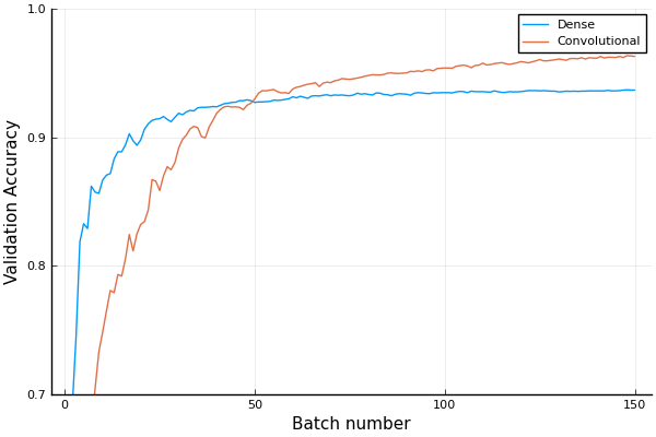
In this case model2 appears better and this agrees with the general fact that convolutional networks train faster and yield better performance for image data.
5.4.4 An ‘industrial strength’ architecture
Here is the VGG19 architecture.
using Metalhead

#downloads about 0.5Gb of a pretrained neural network from the web
vgg = VGG19();
for (i,layer) in enumerate(vgg.layers)
    println(i,":\t", layer)
end
More on these common archictures below. For now just consider the structure of this architecture which has \(19\) layers.
Observe that the number of layers with trained parameters is \(19\) (ignore max pooling, dropout, softmax, and #44 which stands for a reshape function). See the source code.
The number of neurons \(25,088\) is determined by the flow in the first 16 convolutional layers and by the fact that the input is a \(224 \times 224 \times 3\) (image). However the number of neurons \(4096\) is more arbitray.
The number of output neurons is \(1000\) as this network is designed to classify one of \(1000\) labels as specified by the image net challange.
When you do ‘transfer learning’ (more on this in Unit 6), you may use a pretrained model for the convolutional layers and retrain the dense layers at the end.
1:  Conv((3, 3), 3=>64, relu)
2:  Conv((3, 3), 64=>64, relu)
3:  MaxPool((2, 2), pad = (0, 0, 0, 0), stride = (2, 2))
4:  Conv((3, 3), 64=>128, relu)
5:  Conv((3, 3), 128=>128, relu)
6:  MaxPool((2, 2), pad = (0, 0, 0, 0), stride = (2, 2))
7:  Conv((3, 3), 128=>256, relu)
8:  Conv((3, 3), 256=>256, relu)
9:  Conv((3, 3), 256=>256, relu)
10: Conv((3, 3), 256=>256, relu)
11: MaxPool((2, 2), pad = (0, 0, 0, 0), stride = (2, 2))
12: Conv((3, 3), 256=>512, relu)
13: Conv((3, 3), 512=>512, relu)
14: Conv((3, 3), 512=>512, relu)
15: Conv((3, 3), 512=>512, relu)
16: MaxPool((2, 2), pad = (0, 0, 0, 0), stride = (2, 2))
17: Conv((3, 3), 512=>512, relu)
18: Conv((3, 3), 512=>512, relu)
19: Conv((3, 3), 512=>512, relu)
20: Conv((3, 3), 512=>512, relu)
21: MaxPool((2, 2), pad = (0, 0, 0, 0), stride = (2, 2))
22: #44
23: Dense(25088, 4096, relu)
24: Dropout(0.5)
25: Dense(4096, 4096, relu)
26: Dropout(0.5)
27: Dense(4096, 1000)
28: softmax
5.5 Training CNN
Training of convolutional neural networks follows the same paradigm as the training of fully connected neural networks studied in unit 4. The application of a forward pass, and backpropgation yield the gradients and these are then updated using a first order method such as ADAM. The key point is that trained parameters in convolutional layers are the filters and the biases.
All the popular deep learning frameworks, Tensorflow, PyTorch, Keras, Flux (for Julia), and others allow for efficient gradient computation.
A key component of efficient training involves employing GPUs effectively. We do not deal with these aspects in this course. You may enjoy this video by Siraj Raval to get a feel for the usage of GPUs. Then the specific application of GPUs for your purpuse may depend on the language, framework, hardware, and application that you have in mind.
5.6 Four famous architectures
We now survey four famous architectures that were both research landmarks and are used today. The VGG architecture was already used a above. A complete lecture about these architectures is here:
Our purpuse is simply to highlight the key features. See also the Key papers in the development of deep learning section.
- AlexNet: A 2012 network that made history. It has eight layers; the first five are convolutional layers, some of them followed by max-pooling layers, and the last three are fully connected layers. AlexNet used \(11 \times 11\) convolutions in the first layer with a stride of \(4\). It also had an architecture that was taylor made to running on two parallel GPUs (it predates the current deep learning frameworks).
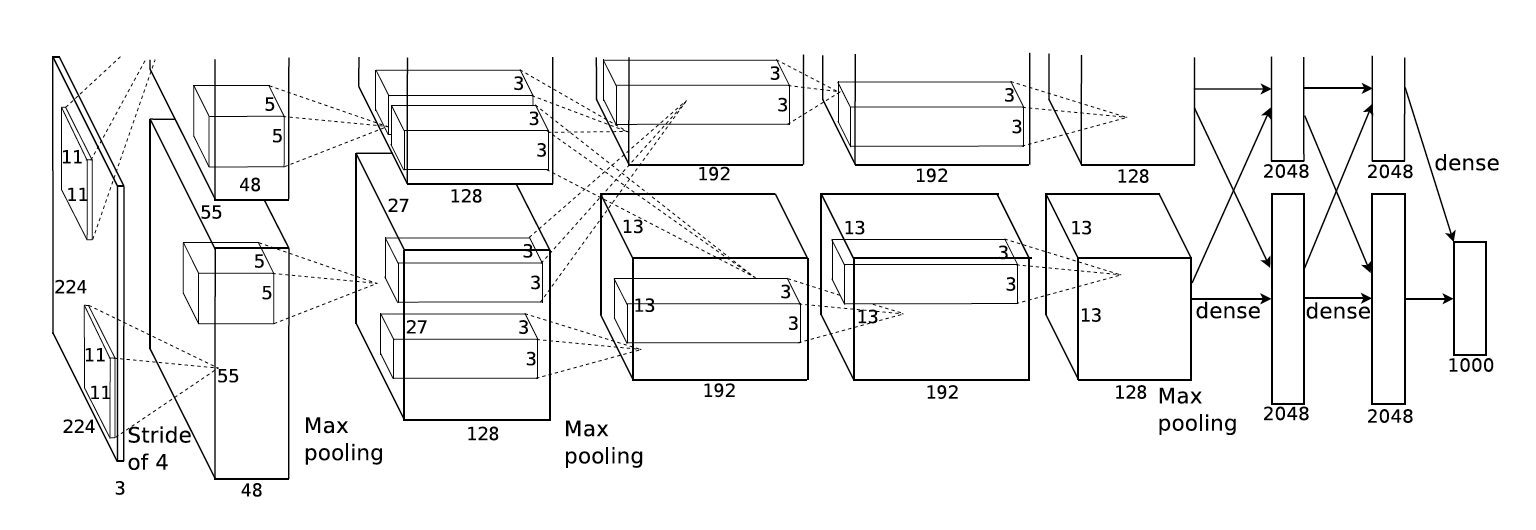
The AlexNet architecture, taken from the original paper
- VGG: This was the next step after AlexNet and is stil used today. Read for example this blog post and see the demonstrations above. A common form is VGG16, but there is also VGG19 that we used above.
Here is a schematic of the VGG19 architecture. Note that the green blocks contain several convolutional layers each.
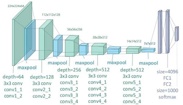
VGG19 - Image courtesy of Clifford K. Yang
To contrast VGG with AlexNet it is useful to consider the concept of the receptive field. The receptive field of a neuron in a CNN is defined as the region in the input space (image) that the neuron is looking at. See for example this comprehnsive blog post. VGG uses combinations to smaller convolutions to achieve similar receptive fields to AlexNet (which uses bigger convolutions).
- Inception (GoogleNet): This network (or better stated as ‘family of networks’) is in many ways close to the current state of the art of general convolutional neural networks. It is heavily used today. See for example this blog post. Key is the usage of inception modules which conctanate seeral convolutional operations together. See for example this short video:
- Resnets: The resnet (residual network) architecture introduces a new idea: residual connections. The main idea is to have layers work on the sum of the output from the direct previous layer as well as several layers back (2 or more). This architecture allows to overcome training problems that occur with very deep networks. Here is a comprehensive video describing Resnets:
5.7 Inner layer interpretation
In general deep learning models and particularly CNNs are not interpretable models. That is, unlike simpler statistical models such as GLMs, the trained parameters of deep neural networks do not have an immediate interpretation.
Nevertheless, the convolutional filters of deep learning networks can be visualized and in certain cases one may make some sense of what certain filters ‘do’. Watch this video which presents several ways for getting some interperation of innner layers.
5.8 Beyond Classification
When learning about CNNs the basic first task to consider is image classification - and this is what we have done above. However, CNNs can be used for several additional important tasks.
These include (among others):
- Object localization: Finding the location (and type) of an object within an image. E.g. looking at an image of a street and identifying cars, pedestrains, and other objects.
- Landmark detection: Finding the location of multiple landmarks within in image. E.g. looking at an image of a face and finding the tip of the nose, the edges of the eyes, etc.
- Object detection: Finding several objects and their type in an image.
- Region proposals: Determining which regions in an image denote different objects.
- One shot learning: A face verification algorithm that uses a limited training set to learn a similarity function that quantifies how different two given images are.
- Style transfer: Transfering style from one type of image to a different type of image.
CNNs have been adapted to deal with tasks such as those above and many others. As an example, one very popular state of the art algorithm that deals with object detection is YOLO (You Only Look Once). See this nice video (again by Siraj Raval):
We don’t cover the full breadth of these tasks in the course, but instaed focus on the simplest task possible, object localization.
5.8.1 Object localization
Here assume you are presented with an image such as this one,

Assume you wish to classify the object in the image as well as to locate where it is in the image. The classification will be to one of \(K\) classes (say “bird”, “plane”, or “nothing”) and the location to a 4-tuple \((x,y,w,h)\) where \((x,y)\) is the location of the top right corner pixel, \(w\) is the width, and \(h\) is the height. The result of such object localization (and classification) may yield something as follows:
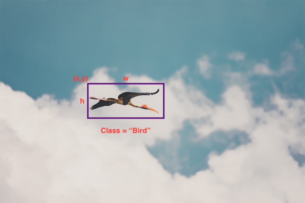
A standard way to carry out this task is to have the network output both the probability vector for the \(K=4\) class labels and the \((x,y,w,h)\) tuple.
A typical way to do this is to have output labels as, \[ y=[p_c, x, y, h, w, p_1,p_2], \] where \(p_c\) indicates the probability that there is an object (0 or 1 on a training image), \(x\), \(y\), \(w\), and \(h\), are as described above, \(p_1\) is the probability of the object (if there is one) being of class 1 (“bird”), and \(p_2\) is the probability of the ojbect (if there is one) beiung of class \(2\) (“plane”).
Note that for images that have “nothing”, the training label will be, \[ y = [0, \emptyset, \emptyset, \emptyset,\emptyset,\emptyset,\emptyset] \] where \(\emptyset\) are ‘don’t care’ values - meaning they can be anything.
Note that we use square loss here for simplicity, however CE loss can be used for the probabilities instead. In this case, a possible training loss is, \[ L(\hat{y},y) = \begin{cases} (\hat{y}_1 - y_1)^2, & \text{if}~\qquad p_c = 0,\\ \sum_{i=1}^7(\hat{y}_i - y_i)^2, & \text{if}~\qquad p_c = 1. \end{cases} \]
Page built: 2021-03-04 using R version 4.0.3 (2020-10-10)