See the latest book content here.
2 Logistic Regression Type Neural Networks
Learning outcomes from this chapter
- Logistic regression view as a shallow Neural Network
- Maximum Likelihood, loss function, cross-entropy
- Softmax regression/ multinomial regression model as a Multiclass Perceptron.
- Optimisation procedure: gradient descent, stochastic gradient descent, Mini-Batches
- Understand the forward pass and backpropogration step
- Implementation from first principles
2.1 Logistic regression view as a shallow Neural Network
2.1.1 Sigmoid function
The sigmoid function \(\sigma(\cdot)\), also known as the logistic function, is defined as follows:
\[\forall z\in\mathbb{R},\quad \sigma(z)=\frac{1}{1+e^{-z}}\in]0,1[\]
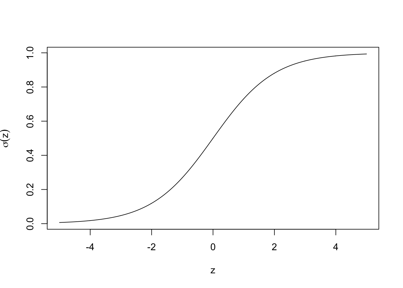 Figure 2.1: Sigmoid function
2.1.2 Logistic regression
The logistic regression is a probabilistic model that aims to predict the probability that the outcome variable \(y\) is 1. It is defined by assuming that \(y|x;\theta\sim\textrm{Bernoulli}(\phi)\). Then, the logistic regression is defined by applying the soft sigmoid function to the linear predictor \(\theta^Tx\):
\[\phi=h_{\theta}(x)=p(y=1|x;\theta)=\frac{1}{1+\exp(-\theta^Tx)}=\sigma(\theta^Tx)\]
The logistic regression is also presented:
\[\textrm{Logit}[h_{\theta}(x)]=logit[p(y=1|x;\theta)]=\theta^Tx\] where \(\textrm{Logit}(p)=log\left(\frac{p}{1-p}\right)\).
Remark about notation
- \(x=(x_0,\dots,x_d)^T\) represent a vector of \(d+1\) features/predictors and by convention \(x_0=1\)
- \(\theta=(\theta_0,\dots,\theta_d)^T\) is the vector of parameter related to the features \(x\)
- \(\theta_0\) is called the intercept by the statistician and named bias by the computer scientist (noted generally \(b\))
2.1.3 Logistic regression for classification
Let’s play with a simple example with 10 points, and two classes (red and blue)
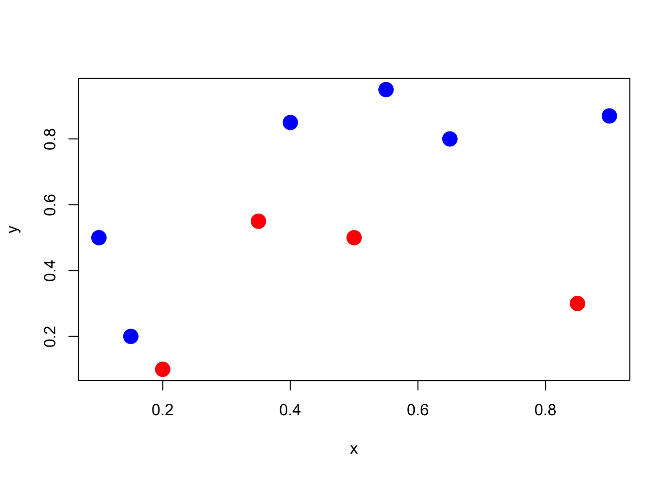 Figure 2.2: Classify red and blue points
clr1 <- c(rgb(1,0,0,1),rgb(0,0,1,1))
clr2 <- c(rgb(1,0,0,.2),rgb(0,0,1,.2))
x <- c(.4,.55,.65,.9,.1,.35,.5,.15,.2,.85)
y <- c(.85,.95,.8,.87,.5,.55,.5,.2,.1,.3)
z <- c(1,1,1,1,1,0,0,1,0,0)
df <- data.frame(x,y,z)
plot(x,y,pch=19,cex=2,col=clr1[z+1])
In order to classify the points, we run a logistic regression to get predictions
Then, we use the fitted model to define our classifier which is defined as attributed the class that is the most likely.
Using our decision rule, we can visualise the produced partition of the space.
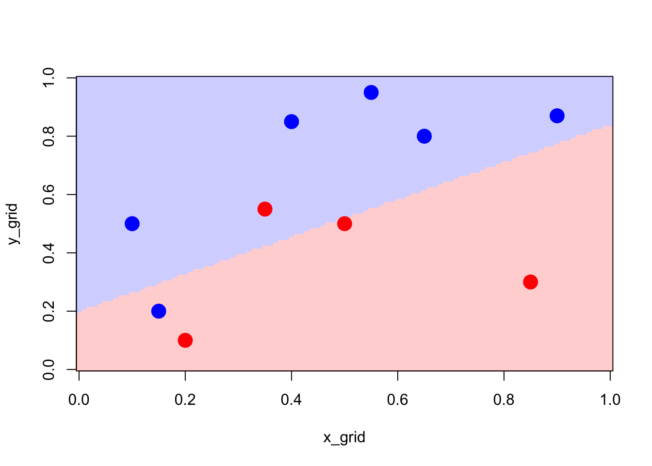 Figure 2.3: Partition using the logistic model
2.1.4 Likelihood of the logistic model
The maximum likelihood estimation procedure is generally used to estimate the parameters of the models \(\theta_0,\ldots,\theta_d\).
\[p(y|x;\theta) = \begin{cases} h_\theta(x) & \text{if } y = 1, \text{ and} \\ 1 - h_\theta(x) & \text{otherwise}. \end{cases}\] which could be written as
\[p(y|x;\theta) = h_\theta(x)^y(1-h_\theta(x))^{1-y},\]
Consider now the observation of \(m\) training samples denoted by \(\left\{(x^{(1)},y^{(1)}),\ldots,(x^{(m)},y^{(m)})\right\}\) as i.i.d. observations from the logistic model. The likelihood is
\[\begin{eqnarray*} L(\theta)&=&\prod_{i=1}^mp(y^{(i)}|x^{(i)};\theta)\\ &=&\prod_{i=1}^m h_\theta(x^{(i)})^y(1-h_\theta(x^{(i)}))^{1-y} \end{eqnarray*}\]
Then, the following log likelihood is maximized to the estimates of \(\theta\):
\[\ell(\theta)=\textrm{log }L(\theta)=\sum_{i=1}^m\left[y^{(i)}\log{h_\theta(x^{(i)})}+(1-y^{(i)})\log{(1-h_\theta(x^{(i)}))}\right] \]
2.1.5 Shallow Neural Network
The logistic model can ve viewed as a shallow Neural Network.
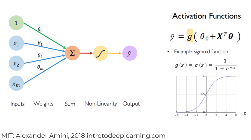
This figure used here the same notation as the regression logistic model presented by the statistical point of view. However, in the following we will adopt the notation used the most frequently in deep learning framework.
Figure 2.4: Shallow Neural Network
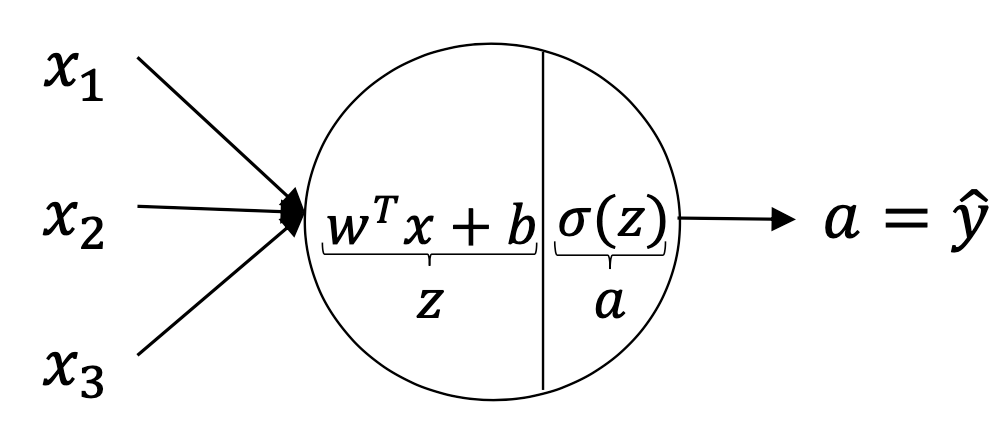
In this figure, \(z=w^Tz+b=w_1x_1+\ldots+w_dx_d+b\) is the linear combination of the \(d\) features/predictors and \(a=\sigma(Z)\) is called the activation function which is the non-linear part of the Neural Network to get a close prediction \(\hat{y}\approx y\).
Remark: In the sequel, we will adopt the following notation:
- \(x=(x_1,\dots,x_d)^T\in \Re^d\) representz a vector of \(d\) features/predictors
- \(w=(w_1,\dots,w_d)^T\) is the vector of weight related to the features \(x\)
- \(b\) is called the biais
- We consider the observations of \(m\) training samples denoted by \(\left\{(x^{(1)},y^{(1)}),\ldots,(x^{(m)},y^{(m)})\right\}\)
2.1.6 Entropy, Cross-entropy and Kullback-Leibler
Let’s first talk about the cross-entropy which is widely used as loss function for classification purpose.
Cross Entropy (CE) is related to the entropy and the kullback-Leibler risk.
The entropy of a discrete probability distribution \(p=(p_1,\ldots,p_n)\) is defined as
\[ H(p)=H(p_1,\ldots,p_n)=-\sum_{i=1}^np_i\log p_i\] which is a ``measurement of the disorder or randomness of a system’’.
Kullback and Leibler known also as KL divergence quantifies how similar a probability distribution \(p\) is to a candidate distribution \(q\).
\[KL(p;q)=-\sum_{i=1}^np_i\log \frac{p_i}{q_i}\] Note that the \(KL\) divergence is not a distance measure as \(KL(p;q)\ne KL(q;p)\). \(KL\) is non-negative and zero if and only if \(p_i = q_i\) for all \(i\).
One can easily show that
\[KL(p;q)=\underbrace{\sum_{i=1}^np_i\log \frac{1}{q_i}}_{\textrm{cross entropy}}-H(p)\]
where the first term of the right part is the cross entropy:
\[CE(p,q)=\sum_{i=1}^np_i\log \frac{1}{q_i}=-\sum_{i=1}^np_i\log q_i\] And we have the relation \[ CE(p,q)=H(p)+KL(p;q)\]
Thus, the cross entropy can be interpreted as the uncertainty implicit in \(H(p)\) plus the likelihood that the distribution \(p\) could have be generated by the distribution \(q\).
2.1.7 Mathematical expression of the Neural Network:
For one example \(x^{(i)}\), the ouput of this Neural Network is given by:
\[\hat{y}^{(i)}=\underbrace{\sigma(w^Tx^{(i)}+b)}_{\underbrace{a^{(i)}}_\textrm{activation function}},\]
where \(\sigma(\cdot)\) is the sigmoid function.
We aim to get the weight \(w\) and the biais \(b\) such that \(\hat{y}^{(i)}\approx y^{(i)}\).
The loss function used for this network is the cross-entropy which is defined for one sample \((x,y)\):
\[\mathcal L(\hat{y},y)=-(y\log \hat{y} + (1-y)\log (1-\hat{y}))\]
Then the Cost function for the entire training data set is:
\[ J(w,b) = \frac{1}{m} \sum_{i=1}^m \mathcal{L}(\hat{y}^{(i)}, y^{(i)})\]
Further, it is easy to see the connection with the log-likelihood function of the logistic model:
\[\begin{eqnarray*} J(w,b) &=& \frac{1}{m} \sum_{i=1}^m \mathcal{L}(\hat{y}^{(i)}, y^{(i)})\\ &=&-\frac{1}{m}\sum_{i=1}^m\left[y^{(i)}\log{a^{(i)})}+(1-y^{(i)})\log{(1-a^{(i)})}\right]\\ &=&-\frac{1}{m}\sum_{i=1}^m\left[y^{(i)}\log{h_\theta(x^{(i)})}+(1-y^{(i)})\log{(1-h_\theta(x^{(i)}))}\right]\\ &\equiv& -\frac{1}{m}\ell(\theta) \end{eqnarray*}\]
where \(b\equiv\theta_0\) and \(w\equiv(\theta_1,\ldots,\theta_d)\).
The optimization step will be carried using Gradient Descent procedures and extension which will be briefly presented in the sub-section Optimization
2.2 Softmax regression
A softmax regression, also called a multiclass logistic regression, is used to generalized logistic regression when there are more than 2 outcome classes (\(k=1,\ldots,K\)). The outcome variable is a discrete variable \(y\) which can take one of the \(K\) values, \(y\in\{1,\ldots,K\}\). The multinomial regression model is also a GLM (Generalized Linear Model) where the distribution of the outcome \(y\) is a Multinomial\((1,\pi)\) where \(\pi=(\phi_1,\ldots,\phi_K)\) is a vector with probabilities of success for each category. This Multinomial\((1,\pi)\) is more precisely called categorical distribution.
The multinomial regression model is parameterize by \(K-1\) parameters, \(\phi_1,\ldots,\phi_K\), where \(\phi_i=p(y=i;\phi)\), and \(\phi_K=p(y=K;\phi)=1-\sum_{i=1}^{K-1}\phi_i\).
By convention, we set \(\theta_K=0\), which makes the Bernoulli parameter \(\phi_i\) of each class \(i\) be such that
\[\displaystyle\phi_i=\frac{\exp(\theta_i^Tx)}{\displaystyle\sum_{j=1}^K\exp(\theta_j^Tx)}\] where \(\theta_1,\ldots,\theta_{K-1} \ \in \Re^{d+1}\) are the parameters of the model. This model is also called softmax regression and generalize the logistic regression. The output of the model is the estimated probability that \(p(y=i|x;\theta)\), for every value of \(i=1,\ldots,K\).
2.2.1 Multinomial regression for classification
We illustrate the Multinomial model by considering three classes: red, yellow and blue.
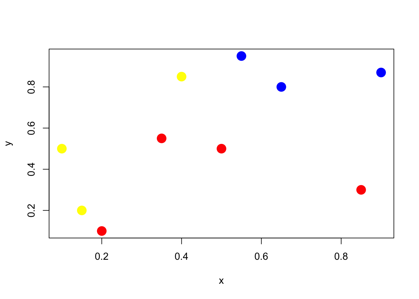 Figure 2.5: Classify for three color points
clr1 <- c(rgb(1,0,0,1),rgb(1,1,0,1),rgb(0,0,1,1))
clr2 <- c(rgb(1,0,0,.2),rgb(1,1,0,.2),rgb(0,0,1,.2))
x <- c(.4,.55,.65,.9,.1,.35,.5,.15,.2,.85)
y <- c(.85,.95,.8,.87,.5,.55,.5,.2,.1,.3)
z <- c(1,2,2,2,1,0,0,1,0,0)
df <- data.frame(x,y,z)
plot(x,y,pch=19,cex=2,col=clr1[z+1])
One can use the R package to run a mutinomial regression model
# weights:  12 (6 variable)
initial  value 10.986123
iter  10 value 0.794930
iter  20 value 0.065712
iter  30 value 0.064409
iter  40 value 0.061612
iter  50 value 0.058756
iter  60 value 0.056225
iter  70 value 0.055332
iter  80 value 0.052887
iter  90 value 0.050644
iter 100 value 0.048117
final  value 0.048117
stopped after 100 iterations
Then, the output gives a predicted probability to the three colours and we attribute the color that is the most likely.
pred_mult <- function(x,y){
res <- predict(model.mult,
newdata=data.frame(x=x,y=y),type="probs")
apply(res,MARGIN=1,which.max)
}x_grid<-seq(0,1,length=101)
y_grid<-seq(0,1,length=101)
z_grid <- outer(x_grid,y_grid,FUN=pred_mult)We can now visualize the three regions, the frontier being linear, and the intersection being the equiprobable case.
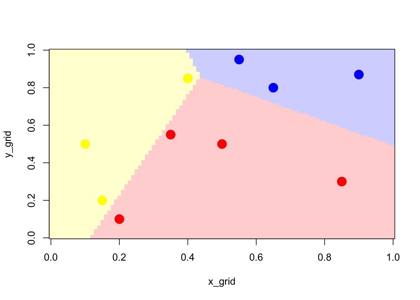 Figure 2.6: Classifier using multinomial model
2.2.2 Likelihood of the softmax model
The maximum likelihood estimation procedure consists of maximizing the log-likelihood:
\[\begin{eqnarray*} \ell(\theta)&=&\sum_{i=1}^m \log{p(y^{(i)|x^{(i)};\theta})}\\ &=&\sum_{i=1}^m\log{\prod_{l=1}^K\left(\frac{e^{\theta_l^Tx^{(i)}}}{\sum_{j=1}^{K}e^{\theta_j^Tx^{(i)}}}\right)^{1_{\{y^{(i)}=l\}}}} \end{eqnarray*}\]
2.2.3 Softmax regression as shallow Neural Network
The Softmax regression model can be viewed as a shallow Neural Network.
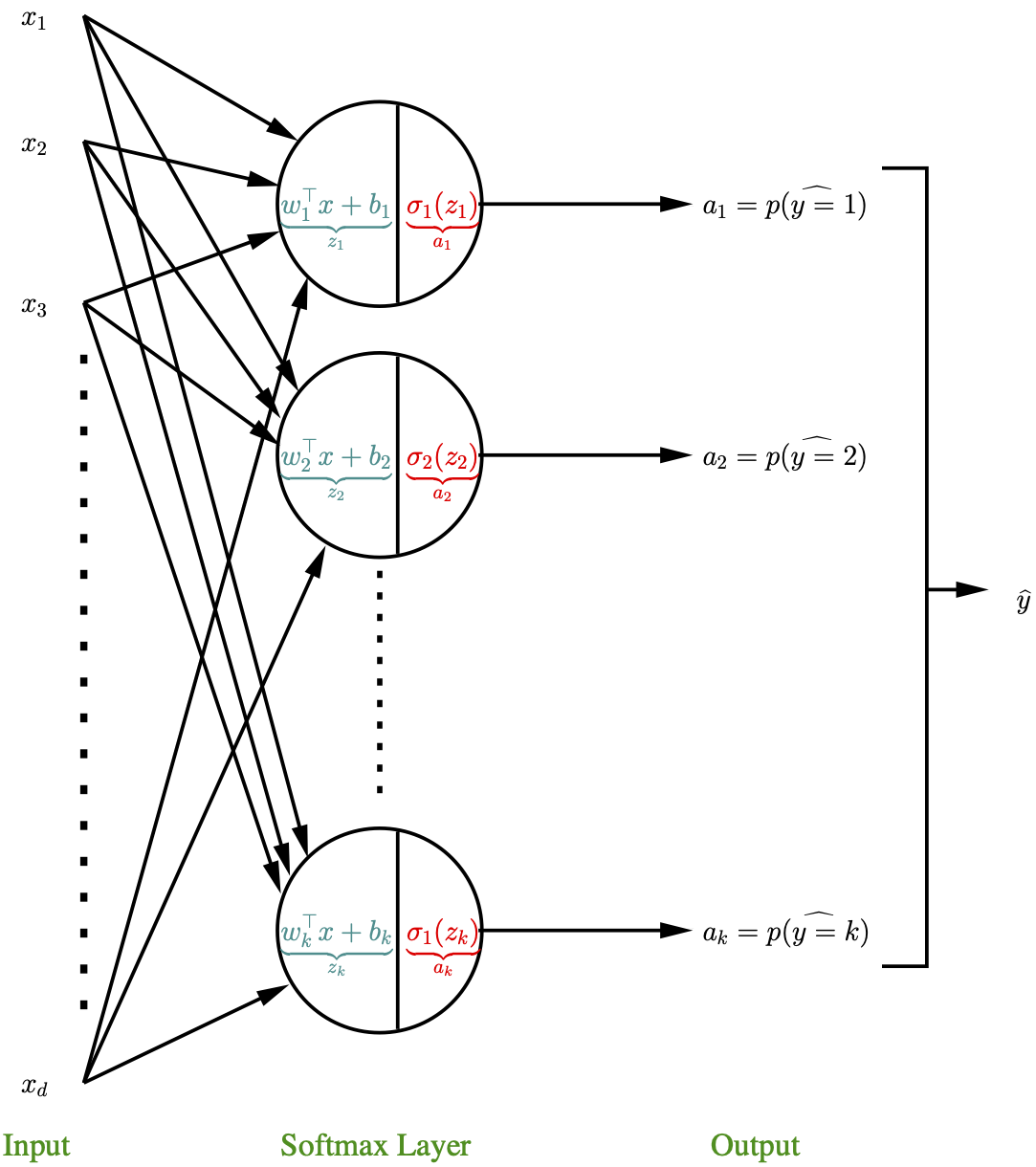
In this representation, there are \(K\) neurons where each neuron is defined by his own set of weights \(w_i \in \Re^d\) and a bais term \(b_i\). The linear part is denoted by \(z_i=w_i^Tx+b_i\) and the non linear part (activation part) is \(\sigma_i=a_i=\frac{\exp(z_i)}{\displaystyle\sum_{j=1}^K\exp(z_j)}\). Note that the denominator of the activation part is defined using the weights from the other neurons. The output is a vector of probabilities \((a_1,\ldots,a_K)\) and the function is used for classification purpose:
\[\boxed{\hat{y}=\underset{i\in \{1,\ldots,K\}}{\textrm{argmax }\ a_i}}\]
2.2.4 Loss function: cross-entropy for categorical variable
Let consider first one training sample \((x,y)\). The cross entropy loss for categorical response variable, also called Softmax Loss is defined as:
\[\begin{eqnarray*} CE&=&-\sum_{i=1}^K\tilde{y}_i\log p(y=i)\\ &=&-\sum_{i=1}^K\tilde{y}_i\log a_i\\ &=&-\sum_{i=1}^K\tilde{y}_i\log\left(\frac{\exp(z_i)}{\displaystyle\sum_{j=1}^K\exp(z_j)}\right) \end{eqnarray*}\] where \(\tilde{y}_i=1_{\{y=i\}}\) is a binary variable indicating if \(y\) is in the class \(i\).
This expression can be rewritten as
\[\begin{eqnarray*} CE&=&-\log \prod_{i=1}^K\left(\frac{\exp(z_i)}{\displaystyle\sum_{j=1}^K\exp(z_j)}\right)^{1_{\{y=i\}}} \end{eqnarray*}\]
Then, the cost function for the \(m\) training samples is defined as
\[\begin{eqnarray*} J(w,b)&=&-\frac{1}{m}\sum_{i=1}^m\log \prod_{k=1}^K\left(\frac{\exp(z^{(i)}_k)}{\displaystyle\sum_{j=1}^K\exp(z^{(i)}_j)}\right)^{1_{\{y^{(i)}=k\}}}\\ &\equiv&-\frac{1}{m}\ell(\theta) \end{eqnarray*}\]
2.3 Optimisation
2.3.1 Gradient Descent
Consider unconstrained, smooth convex optimization
\[\underset{\theta\in \Re^d}{\text{min}}\ f(\theta), \]
Algorithm : Gradient Descent
- Choose initial point \(\theta^{(0)}\in \mathbb R^d\)
- Repeat \(\theta^{(k+1)}=\theta^{(k)}-\alpha.\nabla f(\theta^{(k)}), \ \ k=1,2,3,\ldots\)
- Stop at some point: \(||\theta^{(k+1)}-\theta^{(k)}||_2^2<\epsilon\)
Here, \(\alpha\) is called the learning rate.
Suppose that we want to find \(x\) that minimizes: \[f(x)=1.2(x-2)^2+3.2\]
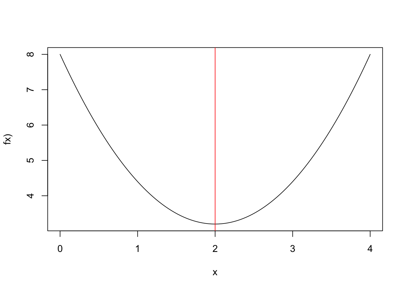 Figure 2.7: Closed from solution (red)
In general, we cannot find a closed form solution, but can compute \(\nabla f(x)\)
simple.grad.des <- function(x0,alpha,epsilon=0.00001,max.iter=300){
  tol <- 1; xold <- x0; res <- x0; iter <- 1
  while (tol>epsilon & iter < max.iter){
    xnew <- xold - alpha*2.4*(xold-2)
    tol <- abs(xnew-xold)
    xold <- xnew
  res <- c(res,xnew)
  iter <- iter +1
  }
 return(res)
}
result <- simple.grad.des(0,0.01,max.iter=200)
#result[length(result)]
Convergence with a learning rate=0.01
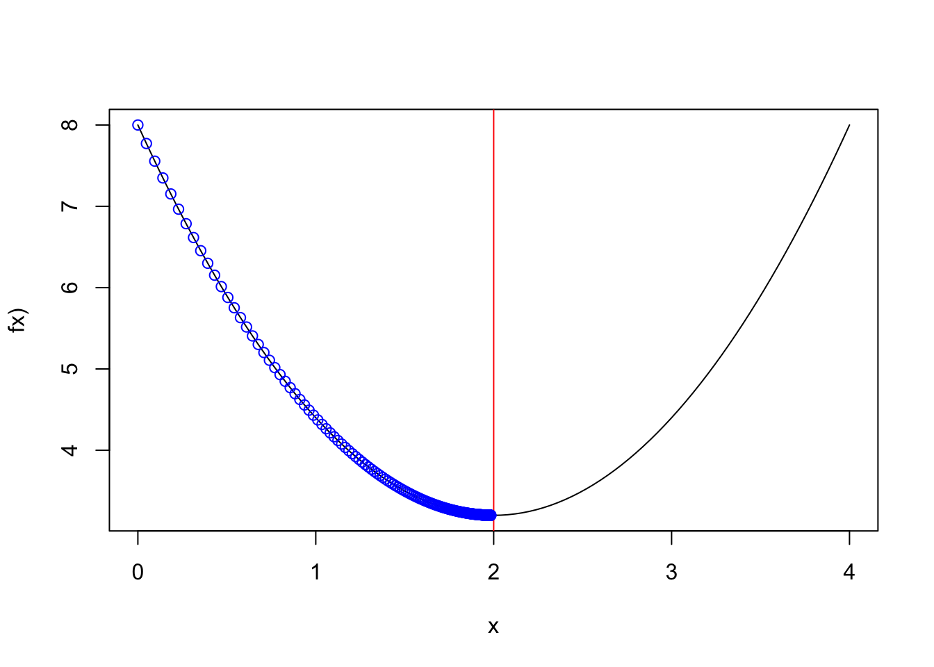 Figure 2.8: alpha=0.01
Convergence with a learning rate=0.83
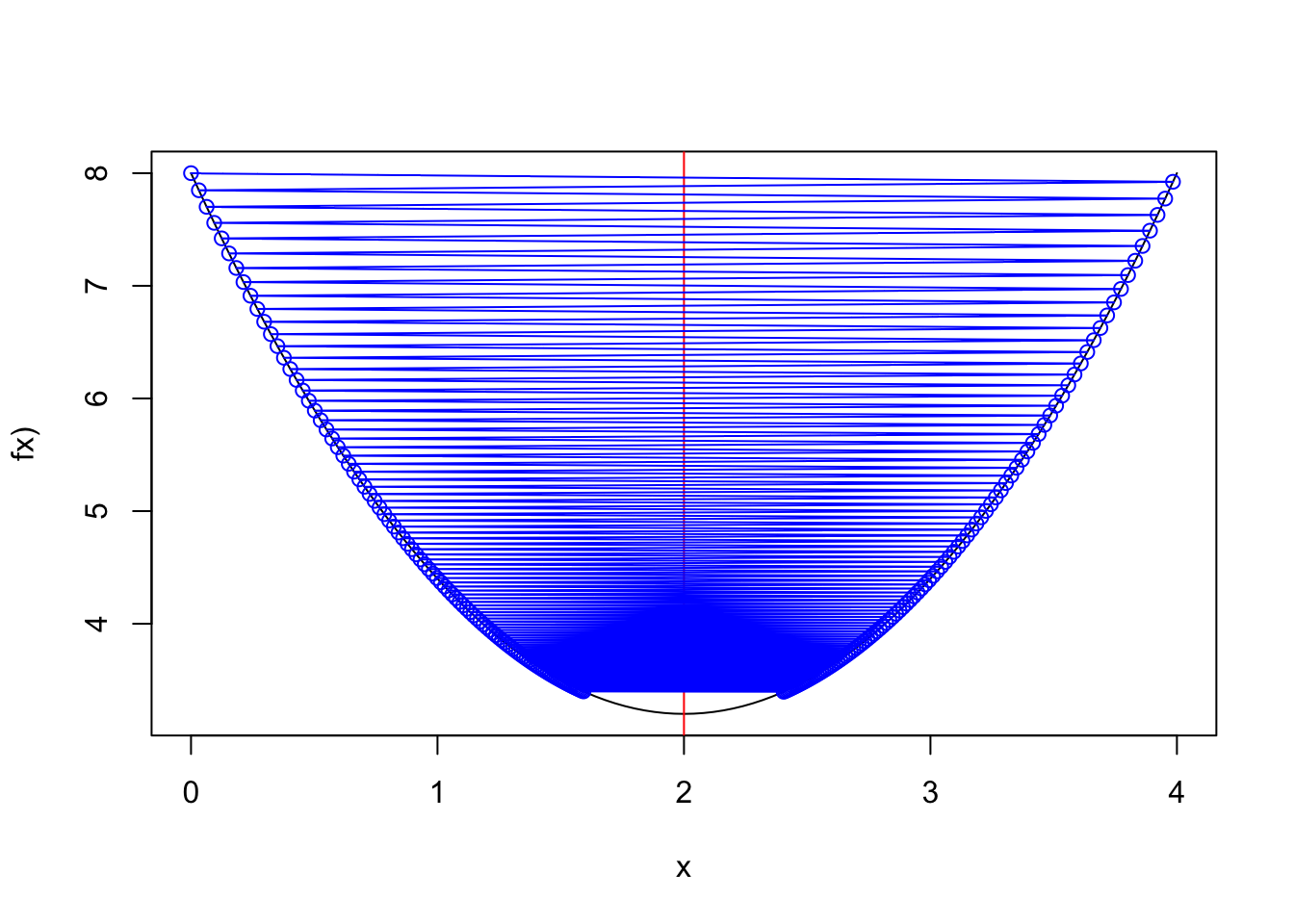 Figure 2.9: alpha=0.83
2.3.2 Gradient Descent for logistic regression
Given \((x^{(i)},y^{(i)})\in \Re\times\{0,1\}\) for \(i=1,\ldots,m\), consider the cross-entropy loss function for this data set:
\[f(w)=\frac{1}{m}\sum_{i=1}^m(-y^{(i)}w^Tx^{(i)}+\log{(1+\exp(w^Tx^{(i)}))})=\sum_{i=1}^mf_i(w)\]
The gradient is
\[\nabla f(w)=\frac{1}{m}\sum_{i=1}^m(p^{(i)}(w)-y^{(i)})x^{(i)}\]
where \[\begin{eqnarray*} p^{(i)}(w))&=&p(Y=1|x^{(i),w})\\ &=&\exp(w^Tx^{(i)})/(1+\exp(w^Tx^{(i)})),\ \ \ i=1,\ldots,m \end{eqnarray*}\]
Algorithm : Batch Gradient Descent
- Initialize \(w=(0,\ldots,0)\)
- Repeat until convergence
- Let \(g=(0,\ldots,0)\) be the gradient vector
- for \(i=1:m\) do \(p^{(i)}=\exp(w^Tx^{(i)})/(1+\exp(w^Tx^{(i)}))\) \(error^{(i)}=p^{(i)}-y_i\) \(g=g+error^{(i)}.w^{(i)}\)
- end
- End repeat until convergence
Note that algorithm uses all samples to compute the gradient. This approach is called batch gradient descent.
2.3.3 Stochastic gradient descent
Algorithm : Stochastic Gradient Descent
Initialize \(w=(0,\ldots,0)\)
-
Repeat until convergence
Pick sample \(i\)
\(p^{(i)}=\exp(w^Tx^{(i)})/(1+\exp(w^Tx^{(i)}))\)
\(error^{(i)}=p^{(i)}-y_i\)
\(w=w-\alpha(error^{(i)}\times x^{(i)})\)
End repeat until convergence
Coefficient \(w\) is updated after each sample.
Remark: The gradient computation \(\nabla f(w)=\sum_{i=1}^m(p^{(i)}(w)-y^{(i)})x^{(i)}\) is doable when \(m\) is moderate, but not when \(m\sim 500 million\).
One batch update costs \(O(md)\)
One stochastic update costs \(O(d)\)
2.3.4 Mini-Batches
In practice, mini-batch is often used to:
- Compute gradient based on a small subset of samples
- Make update to coefficient vector
2.3.5 Example with logistic regression \(d=2\)
- Simulate some \(m\) samples from true model:
\[p(Y=1|x^{(i)},w)=\frac{1}{1+\exp{(-w_1x^{(i)}_1-w_2x^{(i)})}}\]
set.seed(10)
m <- 5000 ;d <- 2 ;w <- c(0.5,-1.5)
x <- matrix(rnorm(m*2),ncol=2,nrow=m)
ptrue <- 1/(1+exp(-x%*%matrix(w,ncol=1)))
y <- rbinom(m,size=1,prob = ptrue)
(w.est <- coef(glm(y~x[,1]+x[,2]-1,family=binomial)))
## x[, 1] x[, 2]
## 0.557587 -1.569509- The cross-entropy loss for this dataset
Cost.fct <- function(w1,w2) {
  w <- c(w1,w2)
  cost <- sum(-y*x%*%matrix(w,ncol=1)+log(1+exp(x%*%matrix(w,ncol=1))))
  return(cost)
}
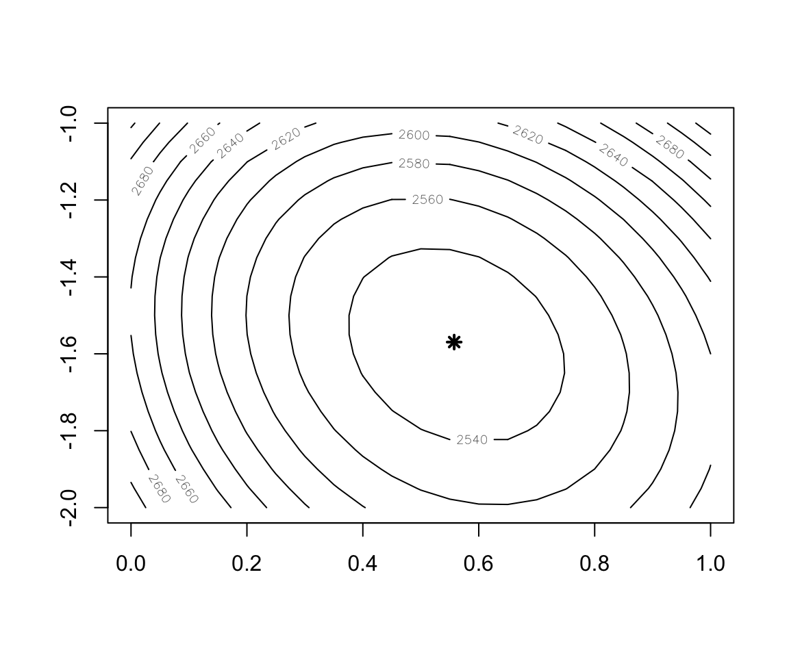 Figure 2.10: Contour plot of the Cost function
w1 <- seq(0, 1, 0.05)
w2 <- seq(-2, -1, 0.05)
cost <- outer(w1, w2, function(x,y) mapply(Cost.fct,x,y))
contour(x = w1, y = w2, z = cost)
points(x=w.est[1],y=w.est[2],col="black",lwd=2,lty=2,pch=8)- Implementation of Batch Gradient Descent
sigmoid <- function(x) 1/(1+exp(-x))

batch.GD <- function(theta,alpha,epsilon,iter.max=500){
  tol <- 1
  iter <-1
  res.cost <- Cost.fct(theta[1],theta[2])
  res.theta <- theta
  while (tol > epsilon & iter<iter.max) {
      error <- sigmoid(x%*%matrix(theta,ncol=1))-y
      theta.up <- theta-as.vector(alpha*matrix(error,nrow=1)%*%x)
      res.theta <- cbind(res.theta,theta.up)
      tol <- sum((theta-theta.up)**2)^0.5
      theta <- theta.up
      cost <- Cost.fct(theta[1],theta[2])
      res.cost <- c(res.cost,cost)
      iter <- iter +1
    }
  result <- list(theta=theta,res.theta=res.theta,res.cost=res.cost,iter=iter,tol.theta=tol)

  return(result)
}## [1] 5000 2## [1] 5000
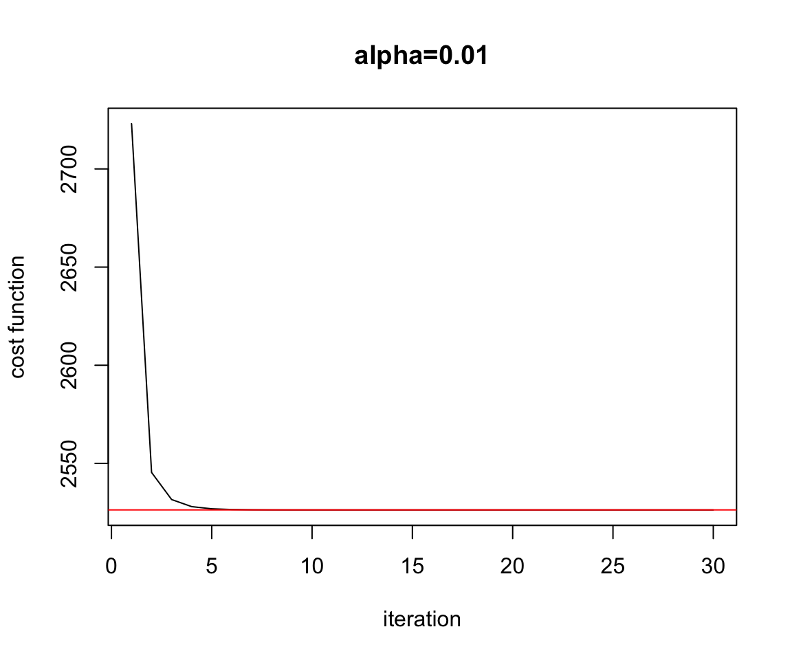 Figure 2.11: Convergence Batch Gradient Descent
theta0 <- c(0,-1); alpha=0.001
test <- batch.GD(theta=theta0,alpha,epsilon = 0.0000001)
plot(test$res.cost,ylab="cost function",xlab="iteration",main="alpha=0.01",type="l")
abline(h=Cost.fct(w.est[1],w.est[2]),col="red")
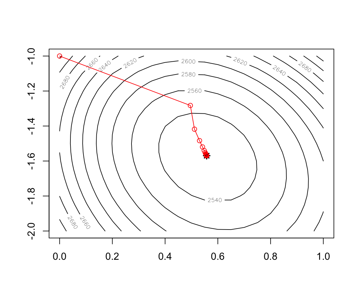 Figure 2.12: Convergence of BGD
contour(x = w1, y = w2, z = cost)
points(x=w.est[1],y=w.est[2],col="black",lwd=2,lty=2,pch=8)
record <- as.data.frame(t(test$res.theta))
points(record,col="red",type="o")- Implementation of Stochastic Gradient Descent
Stochastic.GD <- function(theta,alpha,epsilon=0.0001,epoch=50){
  epoch.max <- epoch
  tol <- 1
  epoch <-1
  res.cost <- Cost.fct(theta[1],theta[2])
  res.cost.outer <- res.cost
  res.theta <- theta
  while (tol > epsilon & epoch<epoch.max) {
    for (i in 1:nrow(x)){
      errori <- sigmoid(sum(x[i,]*theta))-y[i]
      xi <- x[i,]
      theta.up <- theta-alpha*errori*xi
      res.theta <- cbind(res.theta,theta.up)
      tol <- sum((theta-theta.up)**2)^0.5
      theta <- theta.up
      cost <- Cost.fct(theta[1],theta[2])
      res.cost <- c(res.cost,cost)
    }
    epoch <- epoch +1
    cost.outer <- Cost.fct(theta[1],theta[2])
    res.cost.outer <- c(res.cost.outer,cost.outer)
    }
  result <- list(theta=theta,res.theta=res.theta,res.cost=res.cost,epoch=epoch,tol.theta=tol)
}

test.SGD <- Stochastic.GD(theta=theta0,alpha,epsilon = 0.0001,epoch=10)
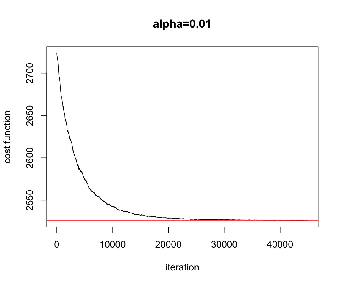 Figure 2.13: Convergence Stochastic Gradient Descent
plot(test.SGD$res.cost,ylab="cost function",xlab="iteration",main="alpha=0.01",type="l")
abline(h=Cost.fct(w.est[1],w.est[2]),col="red")
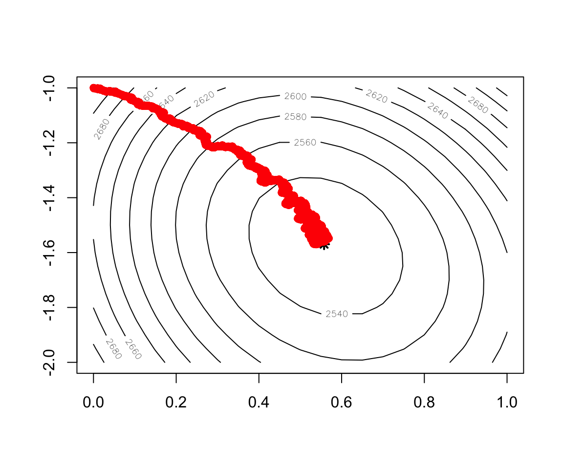 Figure 2.14: Convergence of Stochastic Gradient Descent
contour(x = w1, y = w2, z = cost)
points(x=w.est[1],y=w.est[2],col="black",lwd=2,lty=2,pch=8)
record2 <- as.data.frame(t(test.SGD$res.theta))
points(record2,col="red",lwd=0.5)- Implementation of mini batch Gradient Descent
Mini.Batch <- function (theta,dataTrain, alpha = 0.1, maxIter = 10, nBatch = 2, seed = NULL,intercept=NULL)
{
    batchRate <- 1/nBatch
    dataTrain <- matrix(unlist(dataTrain), ncol = ncol(dataTrain), byrow = FALSE)
    set.seed(seed)
    dataTrain <- dataTrain[sample(nrow(dataTrain)), ]
    set.seed(NULL)

    res.cost <- Cost.fct(theta[1],theta[2])
    res.cost.outer <- res.cost
    res.theta <- theta

    if(!is.null(intercept)) dataTrain <- cbind(1, dataTrain)

    temporaryTheta <- matrix(ncol = length(theta), nrow = 1)
    theta <- matrix(theta,ncol = length(theta), nrow = 1)

    for (iteration in 1:maxIter ) {
        if (iteration%%nBatch == 1 | nBatch == 1) {
            temp <- 1
            x <- nrow(dataTrain) * batchRate
            temp2 <- x
        }
        batch <- dataTrain[temp:temp2, ]
        inputData <- batch[, 1:ncol(batch) - 1]
        outputData <- batch[, ncol(batch)]
        rowLength <- nrow(batch)
        temp <- temp + x
        temp2 <- temp2 + x
        error <- matrix(sigmoid(inputData %*% t(theta)),ncol=1) - outputData
        for (column in 1:length(theta)) {
            term <- error * inputData[, column]
            gradient <- sum(term)#/rowLength
            temporaryTheta[1, column] = theta[1, column] - (alpha *
                gradient)
        }

        theta <- temporaryTheta
        res.theta <- cbind(res.theta,as.vector(theta))
        cost.outer <- Cost.fct(theta[1,1],theta[1,2])
        res.cost.outer <- c(res.cost.outer,cost.outer)

    }
    result <- list(theta=theta,res.theta=res.theta,res.cost.outer=res.cost.outer)
    return(result)
}
theta0 <- c(0,-1); alpha=0.001
data.Train <- cbind(x,y)
test.miniBatch <- Mini.Batch(theta=theta0,dataTrain=data.Train, alpha = 0.001, maxIter = 100, nBatch = 10, seed = NULL,intercept=NULL)
##Result frm Mini-Batch
test.miniBatch$theta## [,1] [,2]
## [1,] 0.5515469 -1.561252
 Figure 2.15: Convergence Mini Batch
plot(test.miniBatch$res.cost.outer,ylab="cost function",xlab="iteration",main="alpha=0.001",type="l")
abline(h=Cost.fct(w.est[1],w.est[2]),col="red")
 Figure 2.16: Convergence of Stochastic Gradient Descent
2.4 Chain rule
The univariate chain rule and the multivariate chain rule are the key concepts to calculate the derivative of cost with respect to any weight in the network. In the following a refresher of the different chain rules.
2.4.1 Univariate Chain rule
- Univariate chain rule
\[\frac{\partial f(g(w))}{\partial w}=\frac{\partial f(g(w))}{\partial g(w)}.\frac{\partial g(w)}{\partial w}\]
2.4.2 Multivariate Chain Rule
- Part I: Let \(z=f(x,y)\), \(x=g(t)\) and \(y=h(t)\), where \(f,g\) and \(h\) are differentiable functions. Then \(z=f(x,y)=f(g(t),h(t)))\) is a function of \(t\), and
\[\begin{eqnarray*} \frac{dz}{dt} = \frac{df}{dt} &=& f_x(x,y)\frac{dx}{dt}+f_y(x,y)\frac{dy}{dt}\\ & = &\frac{\partial f}{\partial x}\frac{dx}{dt}+\frac{\partial f}{\partial y}\frac{dy}{dt}. \end{eqnarray*}\]
- Part II:
- Let \(z=f(x,y)\), \(x=g(s,t)\) and \(y=h(s,t)\), where \(f,g\) and \(h\) are differentiable functions. Then \(z\) is a function of \(s\) and \(t\), and
\[\frac{\partial z}{\partial s} = \frac{\partial f}{\partial x}\frac{\partial x}{\partial s} + \frac{\partial f}{\partial y}\frac{\partial y}{\partial s}\]
and
\[\frac{\partial z}{\partial t} = \frac{\partial f}{\partial x}\frac{\partial x}{\partial t} + \frac{\partial f}{\partial y}\frac{\partial y}{\partial t}\]
- Let \(z = f(x_1,x_2,\ldots,x_m)\) be a differentiable function of \(m\) variables, where each of the \(x_i\) is a differentiable function of the variables \(t_1,t_2,\ldots,t_n\). Then \(z\) is a function of the \(t_i\), and
\[\begin{equation*} \frac{\partial z}{\partial t_i} = \frac{\partial f}{\partial x_1}\frac{\partial x_1}{\partial t_i} + \frac{\partial f}{\partial x_2}\frac{\partial x_2}{\partial t_i} + \cdots + \frac{\partial f}{\partial x_m}\frac{\partial x_m}{\partial t_i}. \end{equation*}\]
2.5 Forward pass and backpropagation procedures
Backpropagation is the key tool adopted by the neural network community to update the weights. This method exploits the derivative with respect to each weight \(w\) using the chain rule (univariate and multivariate rules)
2.5.1 Example with the logistic model using cross-entropy loss
The logistic model can be viewed as a simple neural network with no hidden layer and only a single output node with a sigmoid activation function. The sigmoid activation function \(\sigma(\cdot)\) is applied to the linear combination of the features \(z=w^Tx+b\) and provides the predicted value \(a\) that represent the probability that the input \(x\) belongs to class one.
Figure 2.17: Forward pass: Logistic model
Forward pass: the forward propagation step consists to get predictions for the training samples and compute the error through a loss function in order to further adapt the weights \(w\) and the bias \(b\) to decrease the error. This forward pass is going through the following equations:
\(z^{(i)} = w^Tx^{(i)} + b\)
\(a^{(i)} = \sigma(z^{(i)}) = \frac{1}{1+e^{-z^{(i)}}}\ \ \ i=1,\ldots,m\)
\(L = J(w,b)= -\sum_{i=1}^{m} y^{(i)}\log(a^{(i)}) + (1 - y^{(i)})\log(1-a^{(i)})\)
The cost \(L=J(w,b)\) is the error we want to reduce by adjusting the weights \(w\) and the bais. Variations of the gradient descent algorithm are exploited to update iteratively the parameters. Thus, we have to derive the equations for the gradients on the loss function in order to propagate back the error to adapt the model parameters \(w\) and \(b\).
Backward pass based on computation graph:
The chain rule is used and generally illustrated through a computation graph:
Figure 2.18: backpropagation: Logistic model
First to simplify this illustration, remind that:
\[\begin{eqnarray*} J(w,b) &=& \frac{1}{m} \sum_{i=1}^m \mathcal{L}(\hat{y}^{(i)}, y^{(i)})\\ &=&-\frac{1}{m}\sum_{i=1}^m\left[y^{(i)}\log{a^{(i)})}+(1-y^{(i)})\log{(1-a^{(i)})}\right]\\ \end{eqnarray*}\]
Thus \[\frac{\partial J(w,b)}{\partial w}=\frac{1}{m}\sum_{i=1}^m\frac{\partial \mathcal{L}(\hat{y}^{(i)}, y^{(i)})}{\partial w}\]
To get \(\frac{\partial \mathcal{L}(\hat{y}^{(i)}, y^{(i)})}{\partial w}\) the chain rule is used by considering one sample \((x,y)\) (the notation \(^{(i)}\) is ommitted).
Computation graphs are mainly exploited to show dependencies to derive easely the equations for the gradients. Thus to compute the gradient of the cost (lost function), one only need to go back the computation graph and multiply the gradients by each other:
\[\frac{\partial \mathcal{L}(\hat{y},y)}{\partial w}=\frac{\partial J(w,b)}{\partial a}.\frac{\partial a}{\partial z}.\frac{\partial z}{\partial w}\]
where \(a=\sigma(z)\) and \(z=b+w^Tx\).
- \(\frac{\partial J(w,b)}{\partial a}=-\frac{y}{a}+\frac{1-y}{1-a}=\frac{a-y}{a(1-a)}\)
- \(\frac{\partial \sigma(z)}{\partial z}= \sigma(z)(1- \sigma(z))=a(1-a)\)
- \(\frac{\partial z}{\partial w}= x\)
Thus,
\[\frac{\partial \mathcal{L}(\hat{y},y)}{\partial w}=x(a-y)\]
and so, \[\frac{\partial J(w,b)}{\partial w}=\frac{1}{m}\sum_{i=1}^mx^{(i)}(\sigma(z^{(i)})-y^{(i)})\] In the same vein, it follows
\[\frac{\partial J(w,b)}{\partial b}=\frac{1}{m}\sum_{i=1}^m(\sigma(z^{(i)})-y^{(i)})\]
2.5.2 Updating weights using Backpropagation
For neural network framework, the weights are updated using gradient descent concepts
\[ w = w - \alpha \frac{\partial J(w,b)}{\partial w}\]
The main steps for updating weights are
1. Take a batch of training sample
2. Forward propagation to get the corresponding cost
3. Backpropagate the cost to get the gradients
4. update the weights using the gradients
5. Repeat step 1 to 4 for a number of iterations
2.6 Backpropagation for the Softmax Shallow Network
2.6.1 Remind some notations
We consider \(K\) class: \(y^{(i)}\in \{1,\ldots,K\}\). Given a sample \(x\) we want to estimate \(p(y=k|x)\) for each \(k=1,\ldots,K\). The softmax model is defined by \(\sigma_i=a_i=\frac{\exp(z_i)}{\displaystyle\sum_{j=1}^K\exp(z_j)}\), with \(a_i=p(y=i|x,W)\), \(z_i=b_i+w_i^Tx\) and we write \(W\) to denote all the weights of our network. Then, \(W=(w_1,\ldots,w_K)\) a \(d\times K\) matrix obtained by concatenating \(w_1,\ldots,w_K\) into columns.
2.6.2 Chain rule using cross-entropy loss
Let consider one training sample \((x,y)\). The cross entropy loss is
\[CE=-\sum_{i=1}^K\tilde{y}_i\log a_i\]
where \(\tilde{y}_i=1_{\{y=i\}}\) is a binary variable indicating if \(y\) is in the class \(i\).
To get \(\frac{\partial CE}{\partial w_j}\) (\(j=1,\ldots,K)\) we need to use the multivariate chain rule:
First, we derive
\[\begin{eqnarray*} \frac{\partial CE}{\partial z_j}&=&\sum_{k}^K\frac{\partial CE}{\partial a_k}.\frac{\partial a_k}{\partial z_j}\\ &=&\frac{\partial CE}{\partial a_j}.\frac{\partial a_j}{\partial z_j}-\sum_{k\ne j}^K\frac{\partial CE}{\partial a_k}.\frac{\partial a_k}{\partial z_j} \end{eqnarray*}\]
\(\frac{\partial CE}{\partial a_j}=-\frac{\tilde{y}_j}{a_j}\)
if \(i=j\)
\[\frac{\partial a_i}{\partial z_j}=\frac{\partial\frac{e^{z_i}}{\sum_{k=1}^K e^{z_k}}}{\partial z_j}= \frac{e^{z_i} \left(\sum_{k=1}^K e^{z_k} - e^{z_j}\right)}{\left(\sum_{k=1}^K e^{z_k}\right)^2}=\frac{ e^{z_j} }{\sum_{k=1}^K e^{z_k} } \times \frac{\left( \sum_{k=1}^K e^{z_k} - e^{z_j}\right ) }{\sum_{k=1}^K e^{z_k} }=a_i(1-a_j)\]
- if \(i\ne j\)
\[\frac{\partial a_i}{\partial z_j}=\frac{\partial\frac{e^{z_i}}{\sum_{k=1}^K e^{z_k}}}{\partial z_j}=\frac{0 - e^{z_j}e^{z_i}}{\left( \sum_{k=1}^K e^{z_k}\right)^2}=\frac{- e^{z_j} }{\sum_{k=1}^K e^{z_k} } \times \frac{e^{z_i} }{\sum_{k=1}^K e^{z_k} }=- a_j.a_i\]
So we can rewrite it as
\[\frac{\partial a_i}{\partial z_j} = \left\{ \begin{array}{ll} a_i(1-a_j) & if & i=j \\ -a_j.a_i & if & i\neq j \end{array}\right.\]
Thus, we get
\[\begin{eqnarray*} \frac{\partial CE}{\partial z_j}&=&\frac{\partial CE}{\partial a_j}.\frac{\partial a_j}{\partial z_j}-\sum_{k\ne j}^K\frac{\partial CE}{\partial a_k}.\frac{\partial a_k}{\partial z_j}\\ &=&-\tilde{y}_j(1-a_j)+\sum_{k\ne j}^K\tilde{y}_ja_k\\ &=&-\tilde{y}_j+a_j\sum_{k}^K\tilde{y}_k=a_j-\tilde{y}_j\\ \end{eqnarray*}\]
We can now derive the gradient for the weights as:
\[\begin{eqnarray*} \frac{\partial CE}{\partial w_j}&=&\sum_{k}^K\frac{\partial CE}{\partial z_k}.\frac{\partial z_k}{\partial w_j}\\ &=&(a_j-\tilde{y}_j)x \end{eqnarray*}\]
In the same way, we get
\[\begin{eqnarray*} \frac{\partial CE}{\partial b_j}&=&\sum_{k}^K\frac{\partial CE}{\partial z_k}.\frac{\partial z_k}{\partial b_j}\\ &=&(a_j-\tilde{y}_j) \end{eqnarray*}\]
2.6.3 Computation Graph could help
Let consider a simple example with \(K=3\) (\(y\in\{1,2,3\}\)) and two features (\(x_1\) and \(x_2\)). The computational graph for this softmax neural network model help us to visualize dependencies between nodes and then to derive the gradient of the cost (loss) in respect to each parameter (\(w_j\in\ \Re^{2}\) and \(b_j \in \Re\), \(j=1,2,3\)).
Figure 2.19: Computation Graph: softmax
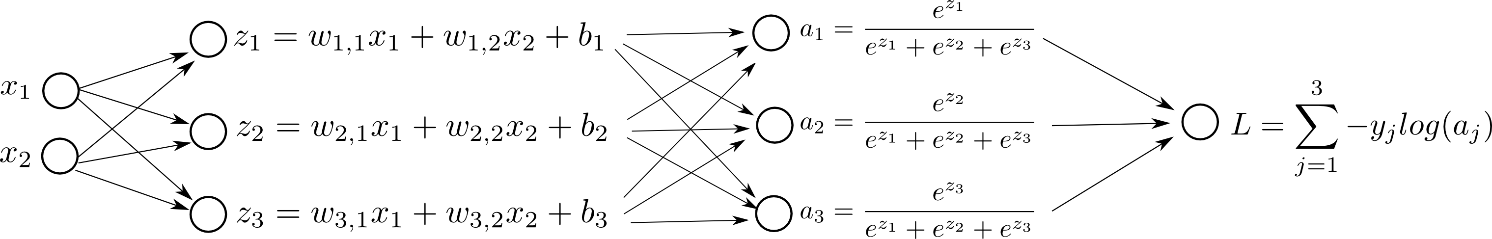
Let’s write as an example for \(\frac{\partial L}{\partial w_{2,1}}\):
\[\begin{align*} \frac{\partial L}{\partial w_{2,1}} & = \sum_{i=1}^3 \left (\frac{\partial L}{\partial a_i} \right) \left (\frac{\partial a_i}{\partial z_2} \right) \left(\frac{\partial z_2}{\partial w_{2,1}} \right ) \\ &= \left (\frac{\partial L }{\partial a_1} \right) \left (\frac{\partial a_1}{\partial z_2} \right) \left(\frac{\partial z_2}{\partial w_{2,1}} \right ) + \left (\frac{\partial L }{\partial a_2} \right) \left (\frac{\partial a_2}{\partial z_2} \right) \left(\frac{\partial z_2}{\partial w_{2,1}} \right ) + \left (\frac{\partial L}{\partial a_3} \right) \left (\frac{\partial a_3}{\partial z_2} \right) \left(\frac{\partial z_2}{\partial w_{2,1}} \right ) \end{align*}\]
In fact, we are summing up the contribution of the change of \(w_{2,1}\) over different “paths” (in red from figure above). When we change \(w_{2,1}\); \(\ a_1\ a_2\) and \(a_3\) changes as a result. Then, the change of \(\ a_1\ a_2\) and \(a_3\) affects \(L\). We sum up all the changes \(w_{2,1}\) produced over \(\ a_1\ a_2\) and \(a_3\) to \(L\).
Page built: 2021-03-04 using R version 4.0.3 (2020-10-10)