See the latest book content here.
9 Deep Reinforcement Learning
In this chapter, we focus on deep reinforcement learning, which is a combination reinforcement learning and deep learning. This combination has enabled machines for solving complex decision problems in robotics, healthcare, finance, automatic vehicle control, to name a few.
Learning outcomes from this chapter:
Markov decision processes
Reinforcement learning
Deep reinforcement learning
9.1 Introduction
Sequential decision making is a key topic in machine learning. In this framework, an agent continuously interacts with and learn from an uncertain environment. A sequence of actions taken by the agent decides how the agent interacts with the environment and learn from it. Sequential decision making finds crucial applications in many domains, including healthcare, robotics, finance, and self-driving cars.
In certain cases decision making processes can be detached from precise details of information retrieval and interaction, and however, in many other practical cases the two are coupled. In the latter case, the agent observes the system, gains information and make decisions simultaneously. This is where techniques such as Markov Decision Processes (MDP), Partially Observable Markov Decision Processes (POMDP), and Reinforcement Learning (RL) play significant roles.
Over the last few years, RL has become increasingly popular in addressing important sequential decision making problems. This success is mostly due to the combination of RL with deep learning techniques thanks to the ability of deep learning to successfully learn different levels of abstractions from data with a lower prior knowledge. Deep RL has created an opportunity for us to train computers to mimic some human solving capabilities.
RL is an interdisciplinary field, addressing problems in
- Optimal control (Engineering)
- Dynamic programming (Operational Research)
- Reward systems (Neuro-science)
- Operant conditioning (Psychology)
In all these different areas of science, there is a common goal to solve the problem of how to make optimal sequential decisions. RL algorithms are motivated from the human decision making based on “rewards provide a positive reinforcement for an action”. This behavior is studied in Neuro-science as reward systems and in Psychology as conditioning.
9.1.1 Applications
Let’s look at some examples where RL plays an important role.
Robitics: Imagine a robot trying to move from point A to point B, starting with a lack of knowledge on its surroundings. In this process, it tries different leg and body moves. From each successful or failed move, it learns and uses this experience in making the next moves.
Vehicle control: Think of you trying to fly a drone. In the beginning you have little or no information on what controls to apply to make a successful flight. As you start applying the controls, you get feedback based on how the drone moving in the air. You use this feedback to decide the next controls.
-
Learning to play games: This is another major area where RL has been very successful recently. You must have heard about Google Deepmind’s Alpha Go defeating world’s best Go player Lee Sedol, or Gerald Tesaro’s software agent defeating world Backgammon Champion. These agents use RL.

Atari Breakout played by Google Deepmind’s Deep Q-learning. To see a video recording of the game, click here. Medical treatment planning: RL finds application in planning medical treatment for a patient. The goal is to learn a sequence of treatments based the patient’s reaction to the past treatments and the patient’s current state. The results of the treatments are obtained only at the end, and hence the decisions need to be taken very carefully as it can be a life and death situation.
Chatbots: Think of Microsoft’s chatbots Tay and Zo, and personal assistants like Siri, Google Now, Cortana, and Alexa. All the agents use RL in improving their conversation with a human user.
9.1.2 Key characteristics
There are some key characteristics that separate RL from the other optimization paradigms and supervised learning methods in machine learning. Some of them are listed below.
No “supervision”: There is no supervisor, no labels telling the agent what is the best action to take. For example, in the robotics example, there is no supervisor guiding the robot in choosing the next moves.
Delayed feedback: Even though there is a feedback after every action, most often the feedback is delayed. That is, the effect of the actions taken by the agent might not be observed immediately. For example, when flying a drone from one point to another, moving it aggressively may seem to be nice as the drone moving towards the target quickly, however, the agent might realize later that this aggressive move made the drone to crash into something.
Sequential decisions: The notion of time is essential in RL: each action effects the next state of the system and that further influences the agent’s next action.
Effects of actions on observations: Another key characteristic of RL is that the feedback the agent obtains is in fact a function of the actions taken by the agent and the uncertainty in the environment. In contrary, for the supervised learning paradigm of machine learning, samples in the training data are assumed to be independent of each other.
9.2 Preliminaries
In this section, we establish some preliminaries that are necessary for understanding the methods discussed later.
9.2.1 Markov chain
Let be a sequence of random objects. We say that the sequence is Markov if for every ,
for any sequence . In other worlds, if indicates time steps, given the current state of a Markov chain, its future is independent of its past.
9.2.2 Contraction mapping
Let be a a mapping on a complete metric space into itself. Any such that is called a fixed point of the mapping . Further, is said to be contraction if there exists a constant such that
for every .
Fixed point theorem is also known as the method of successive approximations or the principle of contraction mappings
Theorem 9.1 (Fixed point theorem): Every contraction mapping defined on a complete metric space has a unique fixed point.
Finding the fixed point is easy: start at an arbitrary point and recursively apply
for each . Then the sequence converges to the unique fixed point.
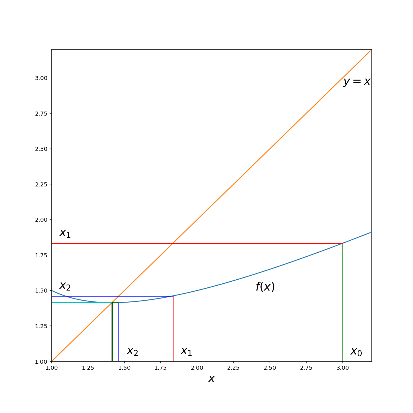
For example consider the following real-valued function on with being the Euclidean distance. It is easy to show that is a contraction mapping with a fixed point at . The following figure illustrates the convergence of the sequence to .
9.3 Markov Decision Processes
To understand RL, we first need to understand the framework of Markov Decision Processes. They are the underlying stochastic models in RL for making decisions. Essentially, RL is the problem we address when this underlying model is either too difficult to solve or unknown in order to find the optimal strategy in advance.
9.3.1 An Example
As a first example, consider a scenario focusing on the engagement level of a student. Assume that there are levels of engagement, , where at level the student is not engaged at all and at the other extreme, at level , she is maximally engaged. Our goal is to maintain engagement as high as possible over time. We do this by choosing one of two actions at any time instant. (0): “do nothing” and let the student operate independently. (1): “stimulate” the student. In general, stimulating the student has a higher tendency to increase her engagement level, however this isn’t without cost as it requires resources.
We may denote the engagement level at (discrete) time by , and for simplicity we assume here that at any time, either increases or decreases by . An exception exists at the extremes of and In these extreme cases the student engagement either stays the same or increases/decreases respectively by . The actual transition of engagement level is random, however we assume that if our action is “stimulate” then there is more likely to be an increase of engagement than if we “do nothing”.
The control problem is the problem of deciding when to “do nothing” and when to “stimulate”. For this we formulate a reward function and assume that at any time our reward is,
Here is some positive constant and if the action at time is to “do nothing”, while if the action is to “stimulate”. Hence the constant captures our relative cost of stimulation effort in comparison to the benefit of a unit of student engagement. We see that depends both on our action and the state.
The reward is accumulated over time into an optimization objective via,
where and is called the discount factor. Through the presence of , future rewards are discounted with a factor of , indicating that in general the present is more important than the future. There can also be other types of objectives, for example finite horizon or infinite horizon average reward, however we only focus on this infinite horizon expected discounted reward case.
A control policy is embodied by the sequence of actions . If these actions are chosen independently of observations then it is an open loop control policy. However, for our purposes, things are more interesting in the closed loop or feedback control case in which at each time we observe the state , or some noisy version of it. This state feedback helps us decide on .
We encode the effect of an action on the state via a family of Markovian transition probability matrices. For each action , we set a transition probability matrix . In our case, as there are two possible actions, we have two matrices such as for example,
Hence for example in state (first row), if we choose action then the transitions follow , whereas if we choose action then the transitions follow . That is for a given state , choosing action implies that the next state is distributed according to (where most of the entries of this probability vector are in this example).
In the case of MDP and POMDP these matrices are assumed known, however in the case of RL these matrices are unknown. The difference between MDP and POMDP is that in MDP we know exactly in which state we are in, whereas in POMDPs our observations are noisy or partial and only hint at the current state. Hence in general we can treat MDP as the basic case and POMDP and RL can be viewed as two variants of MDP. In the case of POMDP the state isn’t fully observed, while in the case of RL the transition probabilities are not known.
We don’t focus on POMDPs further in this course, but rather we continue with MDP and RL. For this, we first need to understand more technical aspects of MDP.
9.3.2 Formal framework
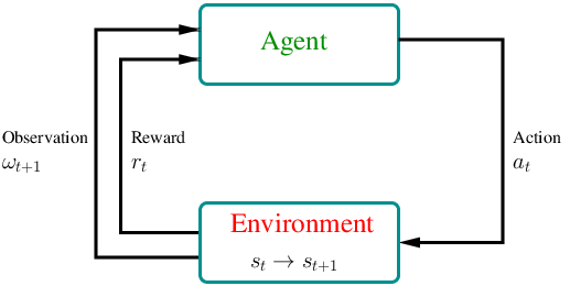
Formally, an MDP is a discrete stochastic control process where the agent starts at time in the environment with an observation about the initial state of the system, where is the space of observations and is the state space. At each time step , (i) the agent obtains a reward with mean , (ii) the state of the system transits from to a new state , and (iii) the agent obtains an observation .
The key property of MDPs is that they satisfy the Markov property, which essentially states that the future is independent of the past given the current observation, and hence the agent has no interest in looking back at the full history.
Definition 9.1 : A descrete time stochastic control process is said to be Markov if for all ,
and
Definition 9.2 : A descrete time stochastic control process is said to be fully observable if for all ,
Definition 9.3 : A Markov Decision Process is a fully observable descrete time stochastic control process which satisfies the Markov property.
An MDP is a 5-tuple , here
is the state space of the system;
is the action space;
is the transition function defining the conditional probabilities between the states;
is the reward function such that for some constant , for all and
is the discount factor;
The agent selects an action at each time step according to a policy . Policies can be divided into stationary and non-stationary. A non-stationary policy depends on time, and they are useful for finite horizon case problems (i.e., there exists a such that the agent takes actions only at ). In this chapter, we consider infinite horizons and stationary policies.
Stationary policies can be further divided into two classes:
Deterministic: There is a unique action for each state specified by a policy map .
Stochastic: The agent takes an action at state according to a probability distribution given by the policy function . Note that for all .
With these notions in mind, we can see that
the transition probability and
the average reward where and
The following figure illustrates the transitions in an MDP.
![]()
9.3.3 Goal of the agent
As in Example 9.3.1, the goal of the agent is to maximize the expected total discounted reward defined by the value function :
where conditioning on implies that at each step, action is selected according to the policy .
Observe that under the stationary assumption, for all ,
Then, the optimal expected return (i.e., optimal value function) is given by
The following result, Theorem 9.2, by (Puterman 1994) states that there exists a deterministic optimal policy that maximizes the value function. That is, the agent has no need to sample action from a probability distribution to achieve maximum expected discounted reward.
Theorem 9.2 (Puterman [1994]): For any infinite horizon discounted MDP, there always exists a deterministic stationary policy that is optimal.
From Theorem 9.2, we can assume that the set of policies contains only deterministic stationary polices.
Further, observe that the action taken by the agent at time determines not only the reward at time , but also the states after time and therefore the rewards after . Hence, the agent has to choose the policy strategically in order to maximize the value function. Now onwards we focus on developing such optimization algorithms.
Exercise: Determine , , , and for Example 9.3.1.
9.3.4 Bellman equations
The following theorem establishes the recursive behavior of the value function: Bellman equations for value functions.
Theorem 9.3 : For any policy ,
Proof. From the definition of the value function,
In particular, for an optimal policy , we have:
Theorem 9.4 : For all ,
where for every pair .
Proof. Observe that, for each ,
If the inequality is strict, we can improve the value of state by using a policy (possibly non-stationary) that uses an action from in the first step.
In fact, (Puterman 1994) shows as a consequence of the fixed point theorem that is a unique solution of (9.5).
In addition to value functions, there are few other functions interests us. Among them most important one is Q-value function defined by
The Q-value is essentially the expected total discounted reward when started in state with initial action , and following policy at each step
Just like the value function, we can show that the Q-value function also satisfies Bellman equation as follows:
Also, similar to value functions, for each pair, the optimal Q-value functions is defined by The main advantage of Q-value function is that the optimal policy can be computed directly from the Q-value function using,
where use some deterministic method to select a solution if is a set.
9.3.5 Iterative algorithms
From the definitions of and , it is immediately obvious that an easy way to estimate them is by using Monte Carlo algorithms, i.e., for each state or each state-action pair , run several simulations starting from or and take sample mean of the values or the Q-values obtained. This is not possible in practice when limited data is available. Even when large data is available, Monte Carlo algorithms may not be computationally efficient compared to the algorithms discussed below.
Assume that both the state space and the action space are finite and discrete. Further assume that the discount factor .
9.3.5.1 Value iteration
It is an indirect method that finds an optimal function , but not optimal policy. In this implementation, we assume that it is easy to compute for any pair .
| Algorithm : Pseudocode for value iteration |
- Start with some arbitrary initial values and fix a small
repeat for until
- For every ,
- Determine optimal policy by
The following theorem establishes that value iteration algorithm convergences to the optimal value. This is again a consequence of the fixed point theorem for contraction mappings.
Theorem 9.5 (Puterman [1994]):
The above algorithm converges linearly at rate :
where .
9.3.5.2 Q-value iteration
Observe that Therefore, the Bellman equations for the Q-value function can be rewritten as follows: The Q-value iteration algorithm below takes advantage of this relation:
| Algorithm : Pseudocode for Q-value iteration |
- Start with some initial Q-values and fix a small
repeat for until
- For every and ,
Similar to the value iteration, since Q-values also satisfy contraction mapping, using the fixed value theorem, we can show that converges to the unique optimal Q-value function linearly.
9.3.5.3 Policy iteration
This is a direct method that finds the optimal policy.
| Algorithm : Pseudocode for policy iteration |
- Start with some initial policy and initial value vector
repeat for until
For every , for all
Set as the value of (compute these values using steps in the value iteration algorithm)
9.3.5.4 Issues with the above three iteration methods
For most practical problems, the state space is higher-dimensional (probably continuous), and the transition probabilities and reward function of the underlying MDP model are either unknown or extremely difficult to compute. For instance, consider the engagement level example, Example 9.3.1. The transition matrices (9.3) and (9.4) are a postulated model of reality. In some situations the parameters of such matrices may be estimated from previous experience, however often this isn’t feasible due to changing conditions or lack of data. So the above iteration algorithms are hard to implement. RL algorithms are useful for solving such problems. We now focus on RL algorithms.
9.4 Reinforcement Learning via Q-Learning
In this section, we explore one class of RL algorithms called Q-learning. The main idea of this method is to learn the Q-function without explicitly decomposing into , and . Observe from the Bellman equation of Q-value function that if we were to know for every state and action , then we can also compute the optimal policy by selecting the that maximizes for every .
The key of Q-learning is to continuously learn while using the learned estimates to select actions as we go. First recall Q-value iteration:
In Q-learning, these updates are approximated using sample observations. As we operate our system with Q-learning, after an action is chosen at time step , the state of the system changes from state to , and a reward is obtained. At that point we update the entry of the Q-function estimate as follows:
Here is a decaying (or constant) sequence of probabilities. A pseudocode of Q-learning is given below.
| Algorithm : Pseudocode for Q-learning |
Input: Given starting state distribution ;
Initialization: Take to be an empty array
repeat for until change in is small
.
Select step sizes
repeat for until epoch is terminated
Select an action .
Observe the next state and the reward .
Take
We attempt to balance exploration and exploitation. With a high probability, we decide on action that maximizes - this is exploitation. However, we leave some possibility to explore other actions, and occasionally decide on an arbitrary (random) action - this is exploration. The key of the Q-learning update equation (9.6) is a weighted average of the previous estimate and a single sample of the right hand side of the Bellman equation of Q-value function. Miraculously as the system progresses under such a control, this scheme is able to estimate the Q-function and hence control the system well.
For the above Q-learning algorithm, the following convergence result holds.
Theorem 9.6 (Watkins and Dayan 1992): Suppose that the rewards are bounded and the learning rates satisfy for all . Let be the estimate of in round .
Then, as almost surely for all where is the instant the action is selected in state .
The above theorem essentially states that if all the actions are selected in all the states infinitely often, and the learning rate decreases to zero but not too quickly, then Q-learning converges. This property shows that (at least in principle), systems controlled via Q-learning may still be controlled in an asymptotically optimal manner, even without explicit knowledge of the underlying transitions .
Issue: It is difficult to implementation of Q-learning algorithm for many practical applications where the state space is large (possibly continuous). There can be many states to visit and keep track of. The following images illustrate this point.
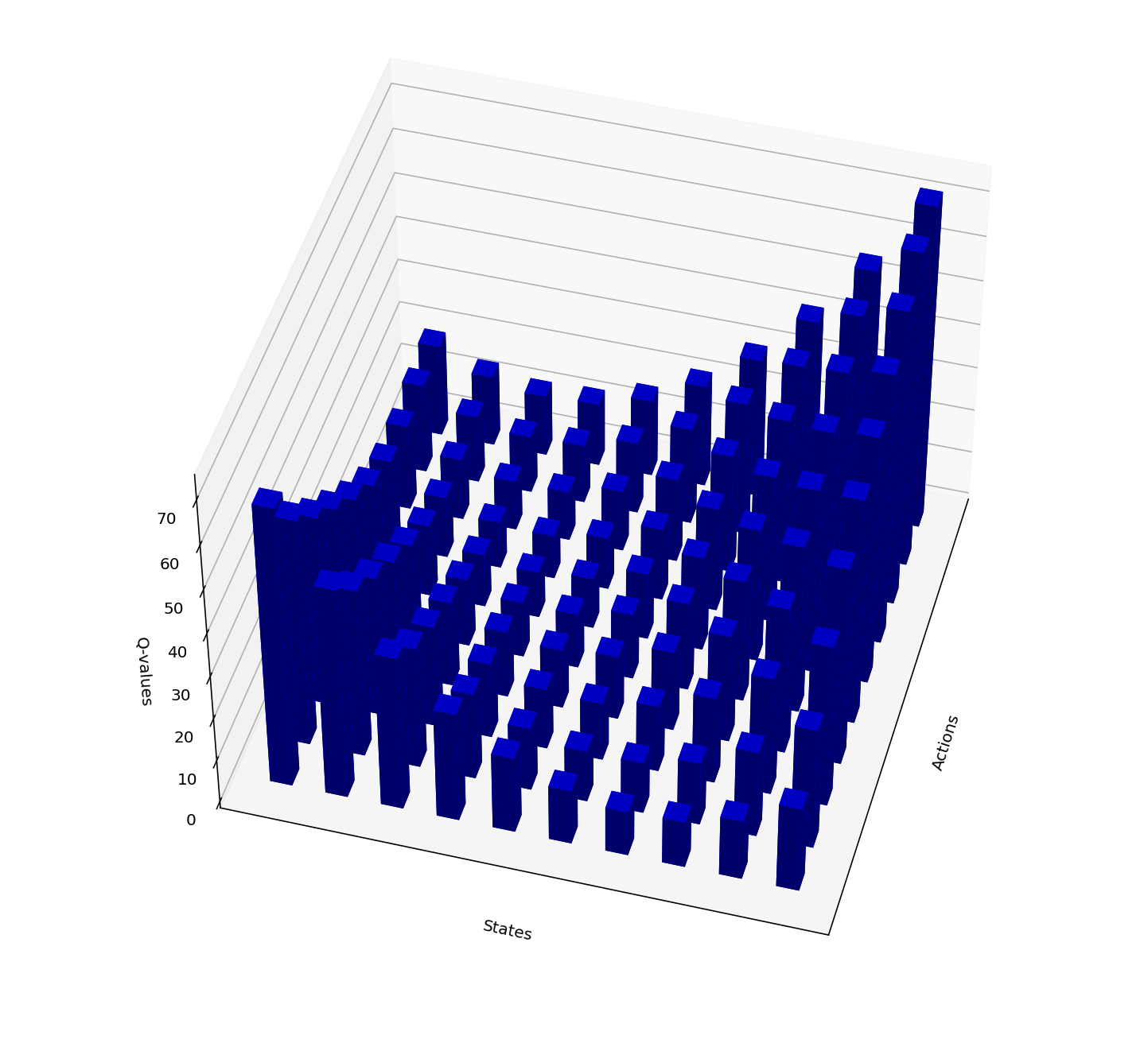
An example of optimal Q-values where neighboring state-action pairs have similar Q-values.
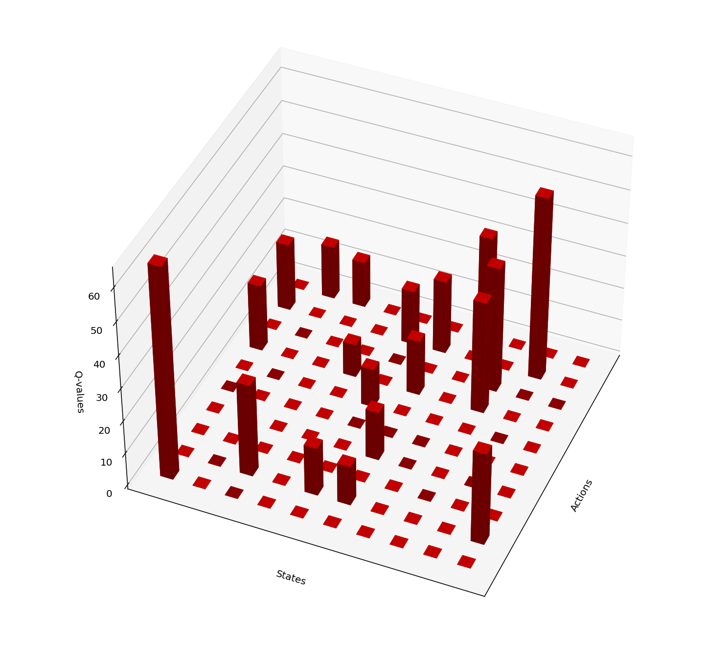
Estimation optimal Q-values using Q-learning. Unexplored state-action pairs carry zero Q-values
9.5 Deep Reinforcement learning
To overcome the scalability issue highlighted above, instead of updating the Q-value of each state-action pair, we would like use what we have learned about already visited states to approximate Q-values of similar states that not yet visited. This is possible even if already visited states are small in number. Deep RL addresses this issue via function approximation using a deep neural network.
The main idea of such methods is to use function approximation to learn a parametric approximation of . For instance, the approximate function can be linear in parameters and features as follows: Or, more generally, we can use a DNN to have an approximation of the form where represents the DNN with parameters (weights, biases). Using such function approximation, for a given , the Q-value function can be computed approximately for unseen state-action pairs . The key point to note that instead of learning matrix of Q-values, function approximation based Q-learning learns . That is, we are trying to find a such that the Bellman equations can be approximated for every state-action pair . We do this approximation by minimizing squares loss function:
Suppose if we take then we are trying to minimize the expectation of The following Q-learning algorithm uses gradient descent to optimize this loss for the observation . When we compare this with supervised learning, acts like actual label and acts like prediction. However, unlike in supervised learning, and are not independent.
| Algorithm : Function approximation based Q-learning |
Fix an initial state
Initiate the parameters
repeat for until the termination condition is satisfied
Start in .
Select step sizes
repeat for until is not a terminal state
Select an action . Probably using the greedy strategy
Observe the next state and the reward .
Take
9.5.1 Deep Q-learning Network (DQN)
In the previous chapters, we have seen several deep neural networks that provide function approximations for models in supervised learning, providing an approximation of the mapping from inputs to the corresponding outputs. Deep Q-learning networks use deep neural networks for the function approximation in the last algorithm, where the parameters are weights and biases of the deep neural network.
9.5.1.1 Key points to note about DQN
In DQN, the input feature at time is formed by the state-action pair . For a given , the output is the prediction for .
Since we do not directly have a target label, we ‘bootstrap’ from the current -network (that is, current parameters ) to generate a target label as .
Then to update the parameters , we use gradient descent on squared loss function.
9.5.1.2 Challenges
Exploration: Recall that the goal is to simultaneously minimize the loss functions . The number of samples available for each depends on how much we explore and . So, there are different number of samples available for different state-action pairs. As a consequence, depending on the transition dynamics of the system, accuracies are different for different pairs. Of course, there is no need to have high accuracy for every state-action pair. For example, rate with low reward can low accuracy without effecting the overall reward. Also, if two state-action pairs have similar features, then it is unnecessary to explore both to learn a good parameter. In summary, it is important to have an adaptive exploration scheme to explore state-action pairs so that the converges of the parameters happens quickly.
Stabilizing: Even though the idea of comparing the prediction to is similar to supervised learning, there are several challenges in deep RL that are not present in supervised learning. Minimizing squared loss is here is different from minimizing loss in supervised learning where ‘true’ labels are present, because is also an estimate that can change too quickly with . As a consequence, the contraction mapping property of Bellman equation may not be sufficient to guarantee convergence of values. There ere experiments suggesting that these errors can propagate quickly, resulting in slow convergence or even making the algorithm unstable. For more details on this, see Section 4 of (François-Lavet et al. 2018) and the references there.
9.5.1.3 Example
The idea of function approximation using neural networks is first proposed in (Mnih et al. 2013) for ATARI games using pixel values as features.
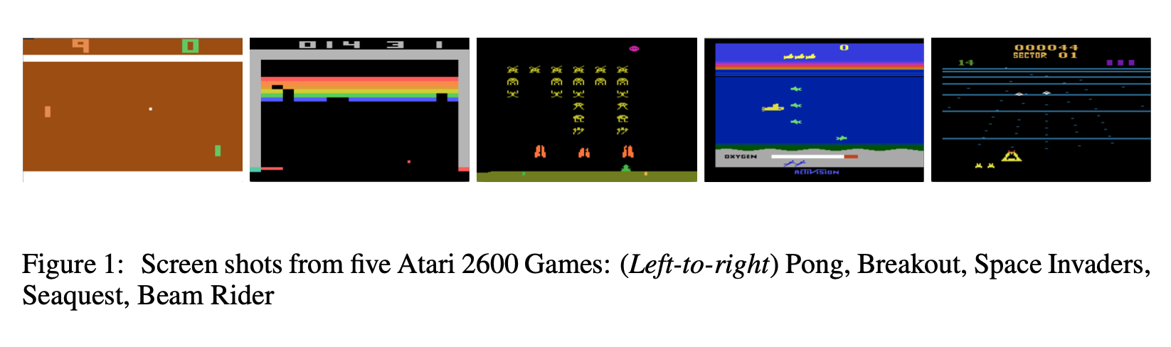
Source: (Mnih et al. 2013)
Essentially, they created a single convolutional neural network (CNN) agent that can successfully learn to play as many ATARI 2600 games as possible. The network was not provided with game specific information or hand-designed visual features. The agent learned to play from nothing but the video input of at . Some specifications of the CNN network used are
Each frame of the video is pre-processed to get an input image of . This is done because working with the original frame size pixels with a color palette is computationally demanding. This process includes first converting the raw RGB frame to greyscale and then down-sampling it to image. Final cropping to the size focuses only on playing area of the image.
The first hidden layer has channels with kernel, stride and ReLu activation function.
The second hidden layer has channels with kernel, stride and ReLu activation function.
The final hidden layer is fully connected linear layer with neurons.
The output layer is again a fully connected linear layer with a single out for each action (i.e., the output size is ). For the games considered in this paper, the number of actions varied between and .
Watch the following video explaining the paper (Mnih et al. 2013) in some more details.
9.5.1.4 Heuristics used in (Mnih et al. 2013) to limit the instability
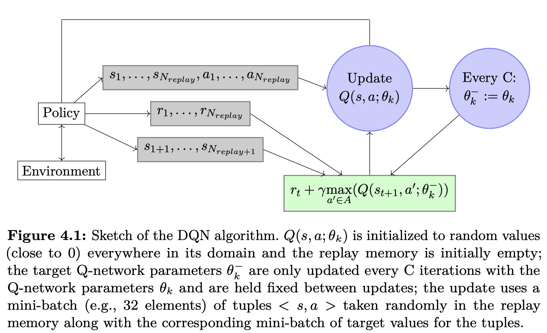
- Note that in the deep Q-learning algorithm the parameters for the is updated after every iterations. This can cause high correlation between the target and the prediction and, as a consequence, instabilities can propagate quickly. To overcome this, (Mnih et al. 2013) updates the parameters of the only after every iterations, while continue to learn the parameters in each iteration. Larger the lesser the correlation. However, if is too large, the parameters in are far from better parameters, creating errors. So, it is important to select a moderate . The following figure illustrates this point (screenshot from (François-Lavet et al. 2018)).
Instead of greedy strategy in selecting an action in each iteration, they use -greedy strategy: selects an action using greedy strategy with probability and selects a random action with probability .
Since the scale of the scores varies from game to game, in addition to the above heuristics, to limit the the scale of error derivatives and make the network easier to use across multiple games, the rewards are clipped as follows: all positive rewards are , all negative rewards are , and rewards are unchanged.
9.5.1.5 Double DQN
The max operation in computing uses the same parameter values to select and evaluate an action. This can result in overestimation of Q-learning values. To remedy this issue, in double DQN (DDQN), the target value is computed as where is the current update and is the current batch update of the parameters.
9.5.1.6 Distributional DQN
So far, in all the methods, the goal is to approximate the expected total discounted reward (either value function or Q-value function). Another richer approach is to find an optimal distribution of the cumulative reward. Such approach provides more information about the randomness of the rewards and transitions of the agent. Suppose is a random variable for each state-action pair with the distribution of cumulative reward obtained under the policy , then it has expectation: for every state-action pair . The recursive relationship for the random reward is given by where and denote the next state and the next action, which are random in nature. Note that .
Recently such distributional DQN are used in practice and they are shown to exhibit additional advantages; refer to (Bellemore et al 2017), (Dabney et al 2017), and (Rowland et al 2018) for more details.
Page built: 2021-03-04 using R version 4.0.3 (2020-10-10)