The ideal network architecture for a task must be found via experimentation guided by monitoring the validation set error.
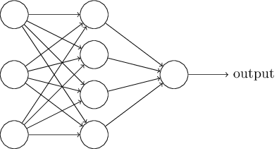
Let’s consider the following architecture.
The left most layer is called the input layer, and the neurons within the layer are called input neurons. A neuron of this layer is of a special kind since it has no input and it only outputs an \(x_j\) value the \(j\)th features.
The right most or output layer contains the output neurons (just one here). The middle layer is called a hidden layer, since the neurons in this layer are neither inputs nor outputs. We do not observe (directly) what goes out of this layer.
Somewhat confusingly, and for historical reasons, such multiple layer networks are sometimes called multilayer perceptrons or MLPs, despite being made up of sigmoid neurons, not perceptrons.
The design of the input and output layers in a network is often straightforward: as many neurons in the input layer than the number of explanatory/features variables; as many neurons in the output layer than the number of possible values for the response variable (if it is qualitative).
But there can be quite an art to the design of the hidden layers. Rectified linear units are an excellent default choice of hidden unit. Rectified linear units are easy to optimize because they are so similar to linear units.
When the output from one layer is used as input to the next layer (with no loops), we speak about feedforward neural networks. Other models are called recurrent neural networks.
Deep feedforward networks, also often called feedforward neural networks,or multilayer perceptrons (MLPs), are the quintessential deep learning models.
4.1.2 Goals
The goal of a feedforward network is to approximate some function \(f^*\). A feedforward network defines a mapping \(y = f(x;\theta)\) and learns the value of the parameters \(\theta\) that result in the best function approximation.
The function \(f\) is composed of a chain of functions: \[f=f^{(k)}(f^{(k-1)}(\ldots f^{(1)})),\] where \(f^{(1)}\) is called the firstlayer, and so on. The depth of the network is \(k\). The final layer of a feedforward network is called the output layer.
Rather than thinking of the layer as representing a single vector-to-vector function, we can also think of the layer as consisting of many unit that act in parallel, each representing a vector-to-scalar function.
Architecture of the network is an art:
how many layers the network should contain
how these layers should be connected to each other
how many units should be in each layer.
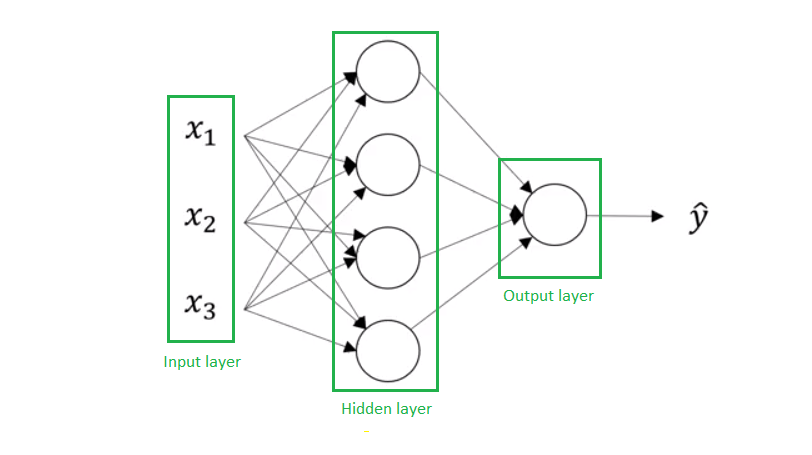
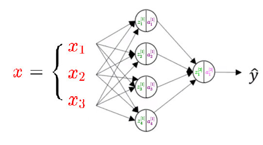
4.1.3 One Layer NN
In this shalow neural network, we have:
\(x_1,\ x_2,\ x_3\) are inputs of a Neural Network. These elements are scalars and they are stacked vertically. This also represents an input layer.
Variables in a hidden layer are not seen in the input set.
The output layer consists of a single neuron only \(\hat{y}\) is the output of the neural network.
\[\left\{
\begin{eqnarray*}
{z^{[1]} } &=& W^{[1]}x +b^{[1]} \\
\hat{y}&=&z^{[2]}=W^{[2]}W^{[1]}x+ W^{[2]}b^{[1]}+b^{[2]}\\
\hat{y}&=&z^{[2]}=W_{new}x+ b_{new}\\
\end{eqnarray*}\right.\]
The output is then a linear combination of a new weight matrix, input and a new bias. Thus if we use an identity activation function then the Neural Network will output linear output of the input. Indeed,a composition of two linear functions is a linear function and so we lose the representation power of a NN. However, a linear activation function is generally recommended and implemented in the output layer in case of regression.
4.1.4 N layers Neural Network
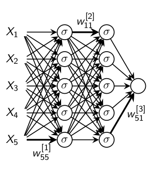
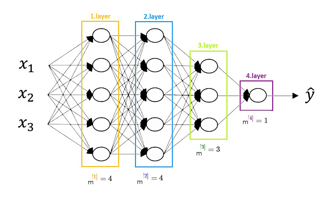
We can generalize this simple previous neural network to a Multi-layer fully-connected neural networks by sacking more layers get a deeper fully-connected neural network defining by the following equations:
This neural network is composed of \(r\) layers based on \(r\) weight matrices \(W^{[1]},\ldots,W^{[r]}\) and \(r\) bias vectors \(b^{[1]},\ldots,b^{[r]}\). The \(r\) activation functions noted \(g^{[r]}\) might be different for each layer \(r\). The number of neurons in each layer could be also be not equal and will be noted \(m_r\). Using this notation:
The total number of neurons in the network: \(m_1+\ldots+m_r\)
Total number of parameters in this network is \((d+1)m_1+(m_1+1)m_2+\ldots+(m_{r-1}+1)*m_r\)
\(W^{[1]}\in\Re^{m_1\times d}\), \(W^{[k]}\in\Re^{m_k\times m_{k-1}}\) (\(k=2,\ldots,r-1\)) and \(W^{[r]}\in\Re^{1\times m_{r-1}}\)
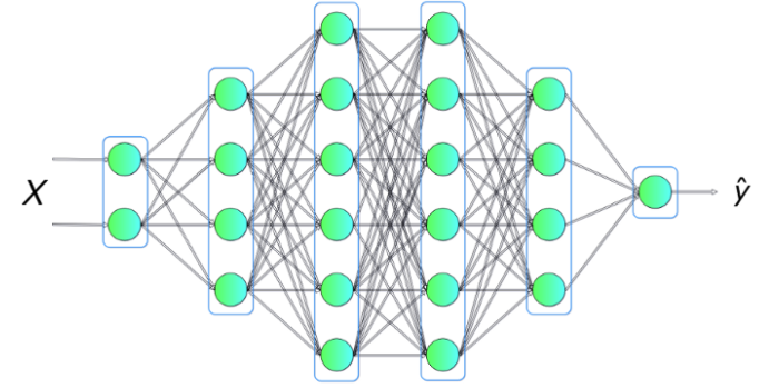
How do we count layers in a neural network?:
When counting layers in a neural network we count hidden layers as well as the output layer, but we don’t count an input layer.
It is a four layer neural network with three hidden layers.
4.1.5 Vectorizing Across Multiple Training Examples
So far we have defined our Neural Network using only one inpute feature vector \(x\) to generate prediction \(\hat{y}\)\[x\longrightarrow a^{[2]}=\hat{y}\]
Let consider \(m\) training example \(x^{[1]},\ldots,x^{[m]}\) and we can use our NN to get for each training example \(x^{[i]}\) a prediction
\[x^{(i)}\longrightarrow a^{[2](i)}=\hat{y}\ \ \ \ i=1,\ldots m\]
One can use a loop for getting all the predictions. However, matrix representation will help us to overcome the computational issue of using loop strategy.
Let first define the matrix \(\textbf{X}\) which every column is a feature vector for one training sample:
Then, we define the matrix \(\textbf{Z}^{[1]}\) with columns \(z^{[1](1)} \ldots z^{[1](m)}\)
\[\textbf{Z}^{[1]} = \begin{bmatrix} \vert & \vert & \dots & \vert \\ z^{[1](1)} & z^{[1](2)} & \dots & z^{[1](m)} \\ \vert & \vert & \dots & \vert \end{bmatrix}.\]
The activation matrix for the first hidden layer \(\textbf{A}^{[1]}\) is defined similary by:
\[\textbf{A}^{[1]}=\begin{bmatrix} \vert & \vert & \dots & \vert \\ a^{[1](1)} & a^{[1](2)} & \dots & a^{[1](m)} \\ \vert & \vert & \dots & \vert\end{bmatrix},\]
where for example the element in the first row and in the first column of a matrix \(\textbf{A}^{[1]}\) is an activation of the first hidden unit and the first training example. For clarification:
\[A^{[1]} = \begin{bmatrix} 1^{st} unit \enspace of \enspace 1.tr. example & 1^{st} unit \enspace of \enspace 2^{nd}tr. example & \dots & 1^{st} unit \enspace of \enspace m^{th}.tr. example \\ 2^{nd}unit \enspace of \enspace 1^{st}tr. example & 2^{nd} unit \enspace of \enspace 2^{nd}tr. example & \dots & 2^{nd} unit \enspace of \enspace m^{th}tr. example \\ the \enspace last \enspace unit \enspace of \enspace 1^{st}tr. example & the \enspace last \enspace unit \enspace of \enspace2^{nd}tr. example & \dots & the \enspace last \enspace unit \enspace of m^{th}tr. example \end{bmatrix}\]
Based on this matrix representation we get:
One can notice that we add \(b^{[1]}\in \Re^{4\times 1}\) to \(W^{[1]}\textbf{X}\in \Re^{4\times m}\), which is strictly not allowed following the rules of linear algebra. In
practice however, this addition is performed using broadcasting. By defining
Leshno and Schocken (1991) has showed that a neural network with one (possibly huge) hidden layer can uniformly approximate any continuous function on a compact set if the activation function is not a polynomial (i.e. tanh, logistic, and ReLU all work, as do sin,cos, exp, etc.).
Let \(\psi(\cdot)\) be any non-polynomial function (an activation function).
Let define \(f:K \longrightarrow \Re\) be any continuous function on a compact set \(K\subset \Re^{m}\)
Then \(\forall \epsilon >0\), there exists an integer \(N\) (the number of hidden units), and parameters \(v_i\), \(b_i\)\(\in \Re\) such that the function
\[F(x)=\sum_{i=1}^{N}v_i\psi(w_i^Tx+b_i)\]
satisfies \(|F(x)-f(x)|>\epsilon\) for all \(x\in K\).
Leshno and Schocken (1991) has noted that this doesn’t work without the bias term \(b_i\). They call it the threshold term.
4.3 Activation function and derivative
Which activation functions to use in the hidden layers ?
Which activation functions to use in the output unit of the Neural Network ?
Let first create a simple plot function for each activation function and its derivative.
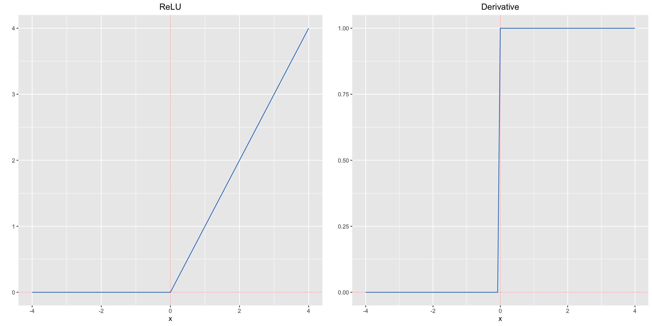
A recent invention which stands for Rectified Linear Units.
\[ReLU(z)=\max{(0,𝑧)}\]
Despite its name and appearance, it’s not linear and provides the same benefits as Sigmoid but with better performance.
Its derivative :
\[\frac{d}{dz}ReLU(z)= \Bigg\{ \begin{matrix} 1 \enspace if \enspace z > 0 \\ 0 \enspace if \enspace z<0 \\ undefined \enspace if \enspace z = 0 \end{matrix}\]
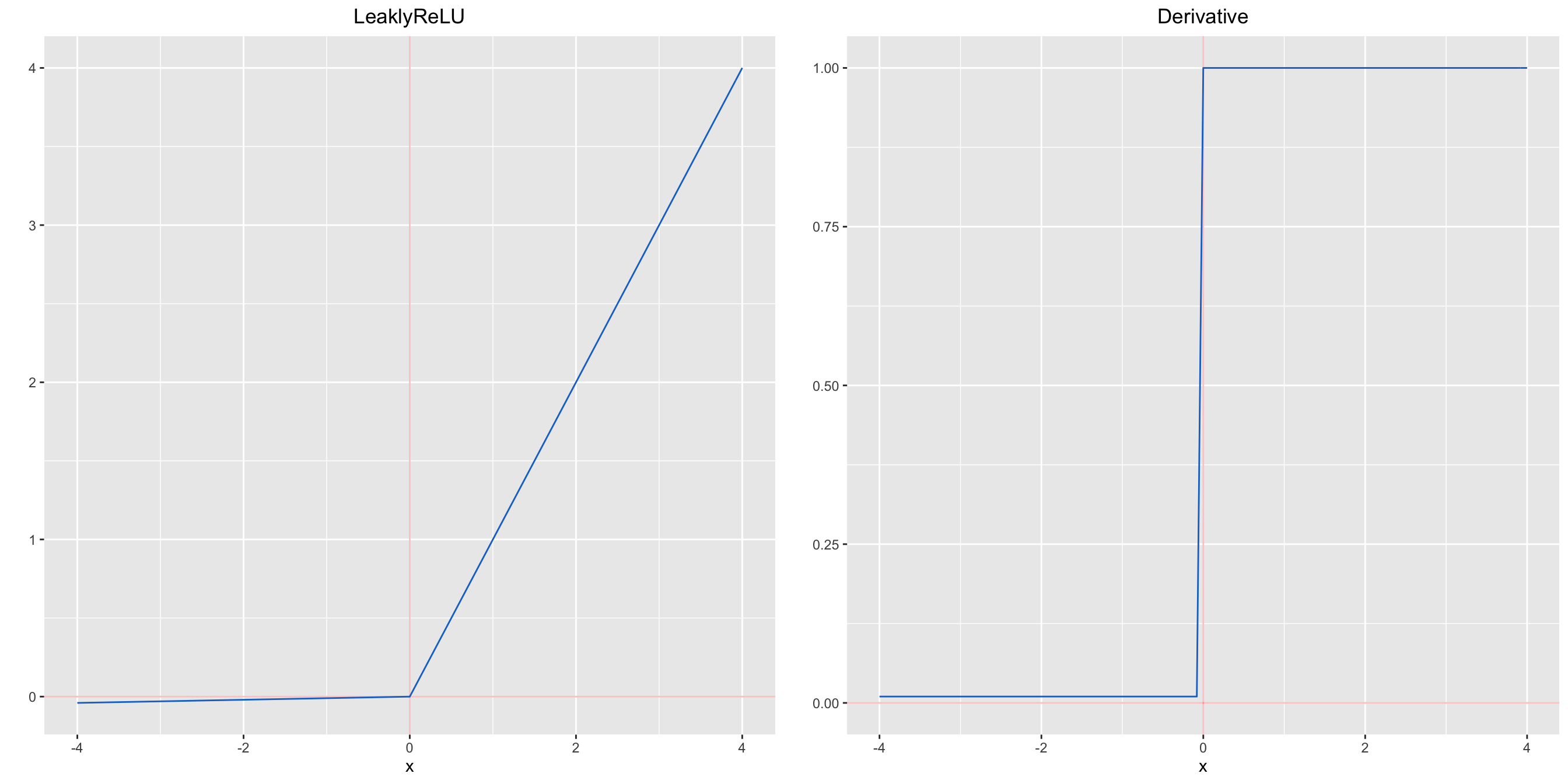
Leaky Relu is a variant of ReLU. Instead of being 0 when \(z<0\), a leaky ReLU allows a small, non-zero, constant gradient \(\alpha\) (usually, \(\alpha=0.01\)). However, the consistency of the benefit across tasks is presently unclear.
\[LeaklyReLU(z)=\max{(\alpha z,𝑧)}\]
Its derivative :
\[\frac{d}{dz}LeaklyReLU(z)= \begin{cases}\alpha & if \ \ z< 0 \\1 & if \ \ z\geq0\\\end{cases}\]
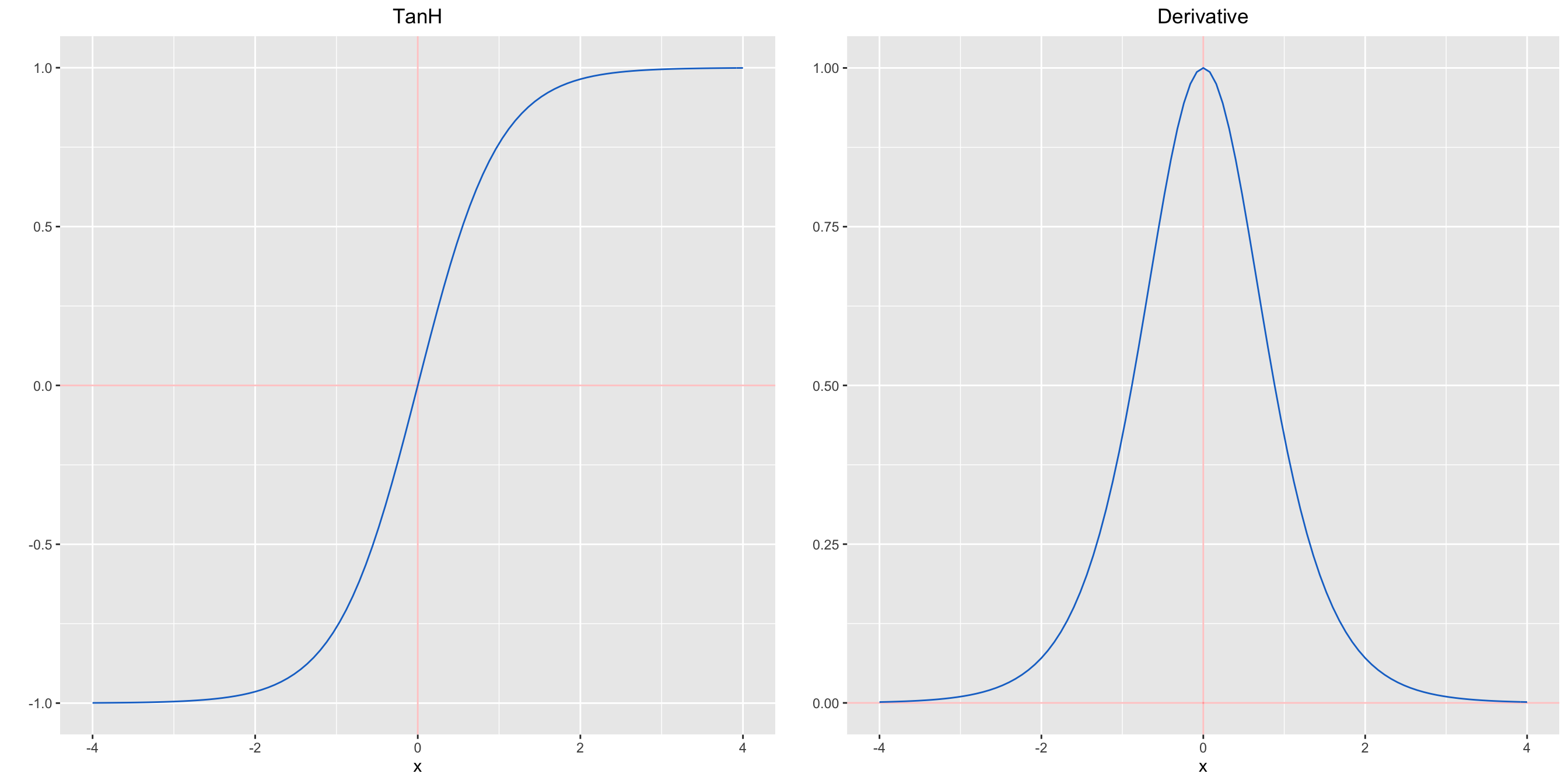
Tanh squashes a real-valued number to the range \([-1, 1]\). It’s non-linear. But unlike Sigmoid, its output is zero-centered. Therefore, in practice the tanh non-linearity is always preferred to the sigmoid nonlinearity.
Let derive the backpropagation algorithm for the following neural network
by considering ReLu activations function for all the neurons of the first Layer and the identity function for the output layer.
Let consider a regression framework and consider the identity function for the output activation function: \(g(x)=x\). In this framework it is natural to use the lesat square cost function:
\[J=\frac{1}{2}(y-\hat{y})^2\]
Let precise some dimension of our objects:
\(d\) is the number of features and \(x\in \Re^d\)
\(m_1\) number of neurons in layer 1 and so \(W^{[1]}\in \Re^{m_1 \times d}\)
\(m_2=1\) number of neurons in output layer and so \(W^{[2]}\in \Re^{1\times m_1}\)
Computing derivatives using Chain Rule using Backward strategy:
-(1) Compute \(\frac{\partial{J}}{\partial W_i^{[2]}}\) then get vectorize version \(\frac{\partial{J}}{\partial W^{[2]}}\)
-(2) Compute \(\frac{\partial{J}}{\partial W_{ij}^{[1]}}\) then get vectorize version \(\frac{\partial{J}}{\partial W^{[1]}}\)
-(3) Compute \(\frac{\partial{J}}{\partial Z_{i}^{[1]}}\) then get vectorize version \(\frac{\partial{J}}{\partial Z^{[1]}}\)
-(4) Compute \(\frac{\partial{J}}{\partial a_{i}^{[1]}}\) then get vectorize version \(\frac{\partial{J}}{\partial a^{[1]}}\)
\[\boxed{
\frac{\partial{J}}{\partial z^{[1]}} = \frac{\partial{J}}{\partial a^{[1]}}\odot \sigma^{'}(z)
}\]
where \(\sigma^{'}(\cdot)\) is the element-wise derivative of the activation function \(\sigma\) (here \(ReLU\) function}) and \(\odot\) denotes the element-wise product of two vectors of the same dimensionality.
First, note that the updated parameter of interests (the weights and bias) depend of intermediate following intermediate variables:
\[z^{[k]}=W^{[k]}a^{[k-1]}+b^{[k]},\ \ \ \ \ k\in\{1,\ldots,r\}\]
Then the cost function depends of weights and bias via the intermediate variables \(z^{[k]}\). Using chain rule we get
Using similar notation as our simple NN, we define \(\delta^{[k]}=\frac{\partial{J}}{\partial z^{[k]}}\)
and compute it in a backward manner from \(k=r\) to 1.
\[\boxed{\delta^{[k]}=\frac{\partial{J}}{\partial z^{[k]}}=\frac{\partial{J}}{\partial a^{[k]}}\odot \textrm{ReLU}^{'}(z^{[k]})}\]
By noting that \(z^{[k+1]}=W^{[k+1]}a^{[k]}+b^{[k+1]}\) and assuming we have computed \(\delta^{[k+1]}\)
then we try to compute \(\delta^{[k]}\). First note that
\[\frac{\partial{J}}{\partial a^{[k]}}=W^{[k+1]T}\frac{\partial{J}}{\partial z^{[k+1]}}\]
then we get
Using our notation, let consider a neural network with \(L\) layer (\(L-1\) hidden layers and \(1\) input and output layer each). The parameter are updated during the training step and are stored in:
\(W^{[l]}\) weight matrix of dimension \(m_{l}\times m_{l-1}\) (\(m_l\) is the size of the layer \(l\))
where the gradients are computed using backpropagation technique
4.5.1 General practice
The biases are initialized with 0 and weights are initialized with random numbers.
What if weights are initialized with 0? or even same constant value
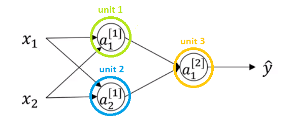
Let consider a neural network with two hidden units and initialize the biases to 0 and all the weights to a constant value \(\gamma\).
By propagating an input sample \((x_1,x_2)\) the output of both hidden units will be the same: \(ReLU(\gamma x_1+\gamma x_2)\). This will have identical influence on the cost function, which will lead to identical gradients. Thus, this makes hidden units symmetric and the neural network will perform very poorly.
A nice animation post on the influence of the weight initialization could be found here Initializing neural networks
Random initialization enables us to break the symmetry. However, initializing much high or low value can result in slower optimization. In practice the natural the weights are randomly gerenated from standard normal distribution. However, while working with a (deep) network can potentially lead to 2 issues: vanishing gradients or exploding gradients.
Vanishing gradients In case of deep networks, for any activation function, \(|\frac{\partial J}{\partial W^{[l]}}|\) will get smaller and smaller as we go backwards with every layer during back propagation. The earlier layers are the slowest to train in such a case. Thus, the update is minor and results in slower convergence. This makes the optimization of the loss function slow. In the worst case, this may completely stop the neural network from training further.
More specifically, in case of \(sigmoid(z)\) and \(tanh(z)\), if your weights are large, then the gradient will be vanishingly small, effectively preventing the weights from changing their value. This is because abs(dW) will increase very slightly or possibly get smaller and smaller every iteration. With \(ReLU(z)\) vanishing gradients are generally not a problem as the gradient is 0 for negative (and zero) inputs and 1 for positive inputs
Exploding gradients This is the exact opposite of vanishing gradients. Consider you have non-negative and large weights. When these weights are multiplied along the layers, they cause a large change in the cost. Thus, the gradients are also going to be large. This means that the changes in \(W^{[l]}\) will be in huge steps. This may result in oscillating around the minima or even overshooting the optimum again and again and the model will never learn!
Another impact of exploding gradients is that huge values of the gradients may cause number overflow resulting in incorrect computations or introductions of NaN’s. This might also lead to the loss taking the value NaN
4.5.2 Solution
For networks that are not too deep, ReLU or leaky RELU activation functions are exploited, as they are relatively robust to the vanishing/exploding gradient issue. In the case of leaky RELU’s, they never have 0 gradient. Thus they never die and training continues.
For deep networks,heuristic to initialize the weights depending on the non-linear activation function are generally used. The most common practice is to draw the element of the matrix \(W^{[l]}\) from normal distribution with variance \(k/m_{l-1}\), where \(k\) depends on the activation function. While these heuristics do not completely solve the exploding/vanishing gradients issue, they help mitigate it to a great extent.
for \(ReLU\) activation: \(k=2\)
for \(tanh\) activation: \(k=1\). The heuristic is called Xavier initialization. It is similar to the previous one, except that \(k\) is 1 instead of 2.
Another commonly used heuristic is to draw from normal distribution with variance \(2/(m_{l-1}+m_l)\)
Note also that Gradient Clipping is another way of dealing with the exploding gradient problem.
Finally, the bias terms can be safely initialized to 0 as the gradients with respect to bias depend only on the linear activation of that layer, and not on the gradients of the deeper layers.
4.6 Batch-normalization and mini-batch
4.6.1 Normalizing inputs to speed up learning
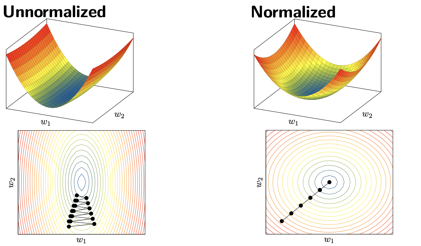
Another common technique in Deep Learning is to normalize the input data. It often leads to a better performance because gradient descent converges faster after normalization.
Note that we also have to use \(\mu_j\) and \(\sigma_j^2\) to normalize validation/test data.
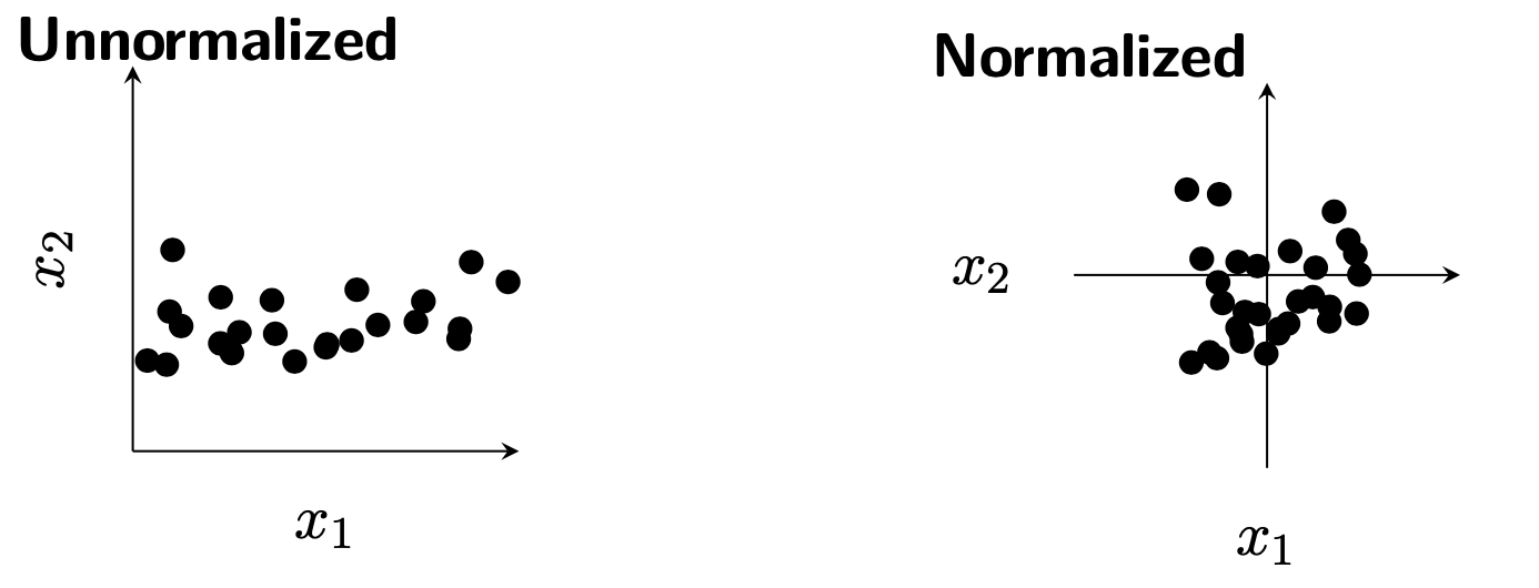
Why normalized the inputs data
For example the inputs \(x_1\) and \(x_2\) are not normalized then the corresponding cost function depending of the parameters \(w_1\) and \(w_2\) can be considered as unormalized. Thus it leads to slower convergence.
4.6.2 Batch Normalization
Not only the input data can be normalized. The inputs of each layer are generally normalized too. This technique is called Batch Normalization (BN). It has been introduced in 2015 and it is one of the most efficient techniques for training deep neural networks. Batch normalization enables to use higher learning rate without getting issues with vanishing or exploding gradients. Moreover, it has also a slight regularization effect.
4.6.3 Batch Normalization on each mini-batch
For every mini-batch, do the following:
Compute mean and variance for every unit \(j\) in all layers \(l\)
\[\mu_j^{(l)}=\frac{1}{m_{batch}}\sum_{i=1}^{m_{batch}}z_j^{(l)[i]},\ \ \ \ (\sigma_j^{(l)})^2=\frac{1}{m}\sum_{i=1}^m(z_j^{(l)[i]}-\mu_j^{(l)})^2\]
where \(z_j^{(l)[i]}\) is the hidden unit before the activation
Normalize every unit \(j\) in all layers \(l\)
\[ \bar{z}_j^{[i]}=\frac{z_j^{(l)[i]}-\mu_j^{(l)}}{\sqrt{(\sigma_j^{(l)})^2+\epsilon}}\]
where \(\epsilon\) is used for numerical stability.
Scale and shift every unit
\[\tilde{z}_j^{[i]}=\gamma_j^{(l)}\bar{z}_j^{[i]}+\beta_j^{(l)}\]
where \(\gamma_l^{(l}\) and \(\beta_j^{(l)}\) are learned parameters ( called batch normalization layer ) that allow the new variable to have any mean and standard deviation.
Why batch normalization ?
The motivation of the prinsep paper is based on internal covariante shift (see for more details Ioffe, Sergey, and Christian Szegedy. ``Batch Normalization: Accelerating Deep Network Training by Reducing Internal Covariate Shift.’’ International Conference on Machine Learning. 2015.arxiv version
It has been recently shown that it makes the loss landscape more smooth and easier to optimize (see Santurkar, Shibani, et al. ”How does batch normalization help optimization?.” Advances in Neural Information Processing Systems. 2018) arxiv version.
4.7 Dropout
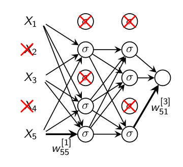
Dropout is a popular and efficient regularization technique.
Dropout is a regularization technique where we randomly drop units.
The term dropout refers to dropping out units (hidden and
visible) in a neural network.
By dropping a unit out, meaning temporarily removed it from the network, along with all its incoming and outgoing connections.
The choice of which units to drop is random.
4.7.1 Main idea
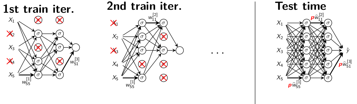
Consider the following network to be trained
1st iteration: Keep and update each unit with probability \(p\), drop remanding ones
2st iteration: Keep and update another random selection of units, drop remanding units.
Continue in the same manner.
Use all units. Weight multiplied by \(p\).
4.7.2 Why does this avoid overfitting?
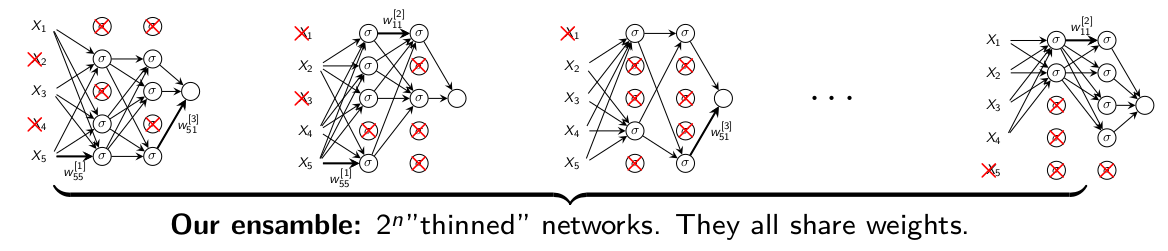
In fact, Dropout can be viewed as an ensemble member with two clever
approximations.
For a neural network with \(M\) units there are \(2^M\) possible
thinned neural networks. Consider this as our ensamble.
Approximation 1: At each iteration we sample one ensemble
member and update it. Most of the networks will never be updated since \(2^M>>\) the number of iterations.
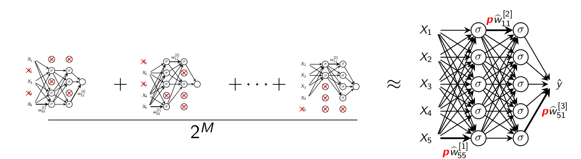
At test time we would need to average over all \(2^M\) which is not
feasible when \(2^M\) is huge.
Approximation 2: Instead, at test time we evaluate the full
neural network where the weight are multiplied by \(p\).
Figure 4.5: Dropout
It has been empirically shown that this is a good approximation of
the average of all ensemble members.
4.8 Basic implementation from first principles
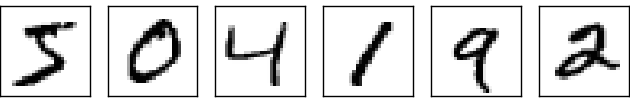
4.8.1 Toy Example: handwritten digits
A simple network to classify handwritten digits
We want to classify images (\(28\times28=784\) pixels) such as these
into 10 classes (0 to 9)
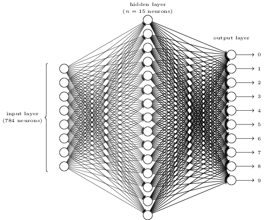
To recognize individual digits we will use a three-layer neural network:
The input pixels are greyscale, with a value of 0.0 representing white, a value of 1.0 representing black, and in between values representing gradually darkening shades of grey.
We number the output neurons from 0 through 9, and figure out which neuron has the highest activation value.
Page built:
2021-03-04
using
R version 4.0.3 (2020-10-10)
 It is a four layer neural network with three hidden layers.
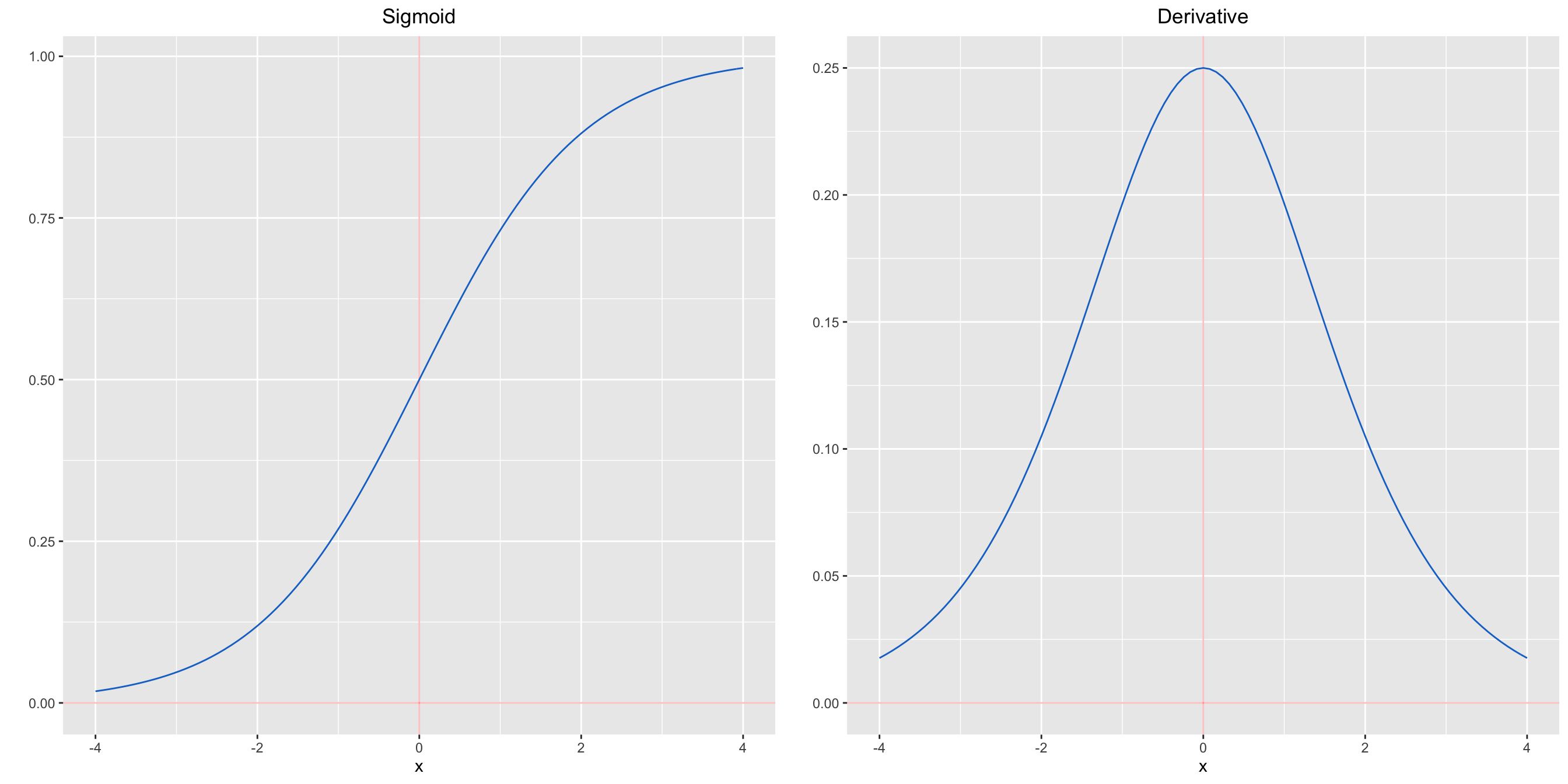
 - Compute mean and variance of training data