See the latest book content here.
7 Generative Adversarial Networks
The world is has some 7.7 billion beautiful people. But in terms of images, infinitly more… Watch this video which shows an advanced application of GANs:
In this unit we overview some of the basics of GANs, a new branch of deep learning that emerged out of a 2014 paper by Ian Goodfellow et. al.
7.1 Generative Models
Generative modelling is an unsupervised learning task in machine learning that involves automatically discovering and learning the regularities or patterns in input data in such a way that the model can be used to generate or output new examples that plausibly could have been drawn from the original dataset.
In general, machine learning distinguishes between the generative approach and the discriminative approach. In the generative approach data such as \(X\) or \((X,Y)\) is used to learn about the probability distribution \(p(X)\) or \(p(X,Y)\). In the discriminative approach we consider the \((X,Y)\) data but learn about the conditional distribution \(P(Y~|~X=x)\).
Logistic regression and the classification and regression neural networks we have used up to now are discriminative. However, some classic machine learning methods are generative. A notable generative model to quickly review is the naive Bayes classifier:
7.1.1 Some classic ML: The Naive Bayes Classifier
Note that naive Bayes is not a Bayesian method.
The Naive Bayes algorithm is not related to GANs or deep learning, but is a classic machine learning (generative) algorithm that is worth knowing.
We have data \(\{(x^{(1)},y_1),\ldots (x^{(n)},y_n)\}\) with \(d\)-vector features and finite labels, say \(\{1,\ldots,K\}\). We assume some family of distributions \(p_\theta(\cdot)\), with parameters \(\theta\), over the data which has a key property (the ‘Naive’ property):
So the key assumption is that the features of \(x\) are condtionally independent given the value of \(y\). \[ p_\theta(x,y) = p_\theta(x ~|~y) p_\theta(y) \underbrace{=}_{\text{Naive}} \Big( \prod_{i=1}^d p_{{\theta}}(x_i~|~y) \Big) p_\theta(y). \]
The naive Bayes algorithm aims to produce a classifier such that with a new observation \({x} \in {\mathbb R}^d\), we have a prediction for the label \(y\). Learning is carried out by estimating \(\hat{\theta}\) from the training data. Then in production/test time, with \(\hat{\theta}\) at hand, prediction is as follows,
This is called the MAP (maximum a posteriori probability) decision rule.
Notice Bayes’ rule.
\[
\begin{array}{rcl}
\hat{y} &=& \text{argmax}_{y \in \{1,\ldots,K\}} p_{\hat{\theta}}(y ~|~x) \\
&=& \text{argmax}_{y \in \{1,\ldots,K\}} \frac{p_{\hat{\theta}}(x ~|~y) p_{\hat{\theta}}(y)}{p_{\hat{\theta}}(x)} \\
&=& \text{argmax}_{y \in \{1,\ldots,K\}} {p_{\hat{\theta}}(x ~|~y) p_{\hat{\theta}}(y)} \\
&=& \text{argmax}_{y \in \{1,\ldots,K\}} \Big( \prod_{i=1}^d p_{\hat{\theta}}(x_i~|~y) \Big) p_{\hat{\theta}}(y) \\
\end{array}
\]
One can now suggest different probability families and use them accordingly. One of the simplest examples which holds when the features are \(\{0,1\}\) boolean is the Bernoulli naive Bayes. Here we assume, \[ p(x ~|~y) = \prod_{i=1}^d p_{yi}^{x_i}(1-p_{yi})^{1-x_i}. \] Hence the parameters \(p_{yi}\), for \(y=1,\ldots,K\) and \(i=1,\ldots,d\) is the probability of class \(y\) generating the term \(x_i\).
Naive Bayes of this sort (and generalizations) has been very popular in e-mail spam detection based on a bag of words summary of the document in question.
7.2 Adverserial Training
Generally, Adversarial machine learning is the collection of techniques that attempt to fool models by supplying deceptive input. Adversarial training includes a variety of methods and applications, many of which are aimed at improving the quality of classifiers or at the same time exposing vulnerabilities.
A famous example is in this video:
More details are in this paper:
2018: Synthesizing robust adversarial examples by Anish Athalye, Logan Engstrom, Andrew Ilyas, and Kevin Kwok.
In the context of GANs, we harness the “adversarial” nature of two sub-models which we train.
7.3 The idea of Generative Adversarial Networks (GAN)
It is ‘different’ from Naive bayes or density estimation methods which attempt to learn about \(p(X,Y)\) directly. A somewhat different type of generative model does not learn about \(p(X)\) or \(p(X,Y)\) but rather learns of a mechanism to generate samples of \(X\) or \((X,Y)\) that follow the same (or similar) distribution to the data. Generative Adversrial Networks (GANs) are such models.
Here we discuss the data as only \(X\), but later we can expand to \((X,Y)\). The basic idea of a GAN is to simultaneously create two models, a generator (\(G\)) and a discriminator (\(D\)). The role of \(G\) is to be a generative model which can transform noise samples \(Z\), (not having any information) also called latent space, into examples of \(X\). The role of \(D\) is to act as a binary classifier between “generated samples” \(G(Z)\) and real samples \(X\). The basic output of training a GAN is \(G(\cdot)\), the generator. In contrast the discriminator is there helping along the way, but is eventually “useless” because once \(G(\cdot)\) is good in generating samples, \(D(\cdot)\) cannot classify between a randomly generated sample \(G(Z)\) and a data sample \(X\).
This image describes the basic architecture well:
The generator \(G\) works on noise vectors from the latent space to create “fake samples”. The discriminator aims to discriminate between real samples of the data and fake samples. The training of \(G\) and \(D\) is simultanious where eventually \(D\) cannot distinguish between “real” and “fake”.

Image from a blog post by Al Gharakhanian.
When we say a generator model \(G(\cdot)\) and a discriminator model \(D(\cdot)\) we assume they each have some (typically) fixed architectures and learned parameters \(\theta_G\) and \(\theta_D\). These are going to be neural networks. so \(\theta_G\) and \(\theta_D\), are the weights, biases, filter parameters, batch-normalization parameters, etc.
7.3.1 Constructing a “game”
In training \(G\) and \(D\) we want an objective that will motivate \(G\) to create better samples and at the same time improve \(D\) in detecting if a sample is from \(G\), or is alternativly a real data sample. To formulate this object lets make use of the two probability distributions that are at play:
We often take the probability distribution of the noise to be an i.i.d. Gaussians distribution of some given dimension (called the latent dimension).
\(p_{\text{data}}(x)\) is the probability distributions of data samples.
\(p_{z}(z)\) is the probability distribution of the noise.
Take \(D(\cdot)\) as a classifier that returns \(1\) for a real image and \(0\) for a fake image. Then the discriminator wants high values of: \[ \mathbb{E}_{X \sim p_{\text {data }}}[\log D(X)]. \]
Further for every \(Z\) we have a fake sample \(G(Z)\) and \(D(G(Z))\) is the discriminators clasification which is ideally \(0\). Hence the discriminator also wants high values of: \[ \mathbb{E}_{Z \sim p_{z}}[\log (1-D(G(Z)))]. \]
Put together for some fixed discriminator \(D(\cdot)\) and fixed generator \(G(\cdot)\) the discriminator wishes to maximize,
\[ V(G,D) :=\mathbb{E}_{X \sim p_{\text {data }}}[\log D(X)] + \mathbb{E}_{Z \sim p_{z}}[\log (1-D(G(Z)))]. \]
Now for any fixed discriminator (parameters/model) that achieves \[ \max_D V(D,G), \] the generator wants to “fool” the discriminator, so it wishes to achieve, \[ \min_G \max_D V(D,G). \]
Since by now there are several other GAN formulations (see below), this type of original GAN formulation is these days refered to as vanilla GAN. This is the basic GAN formulation, formulated as a mini-max game and if we found parameters \(\theta_G\) and \(\theta_D\) such that achieve the “saddle point” \(\min_G \max_D V(D,G)\), then we have trained the GAN.
7.3.2 The basic training loop
Achieving the idealized \(\min_G \max_D V(D,G)\) can be obtained approximately via basic iteration of stochastic gradient descent where \(G\) and \(D\) are trained jointly. The basic algorithm (still from the original GAN paper) is as follows:
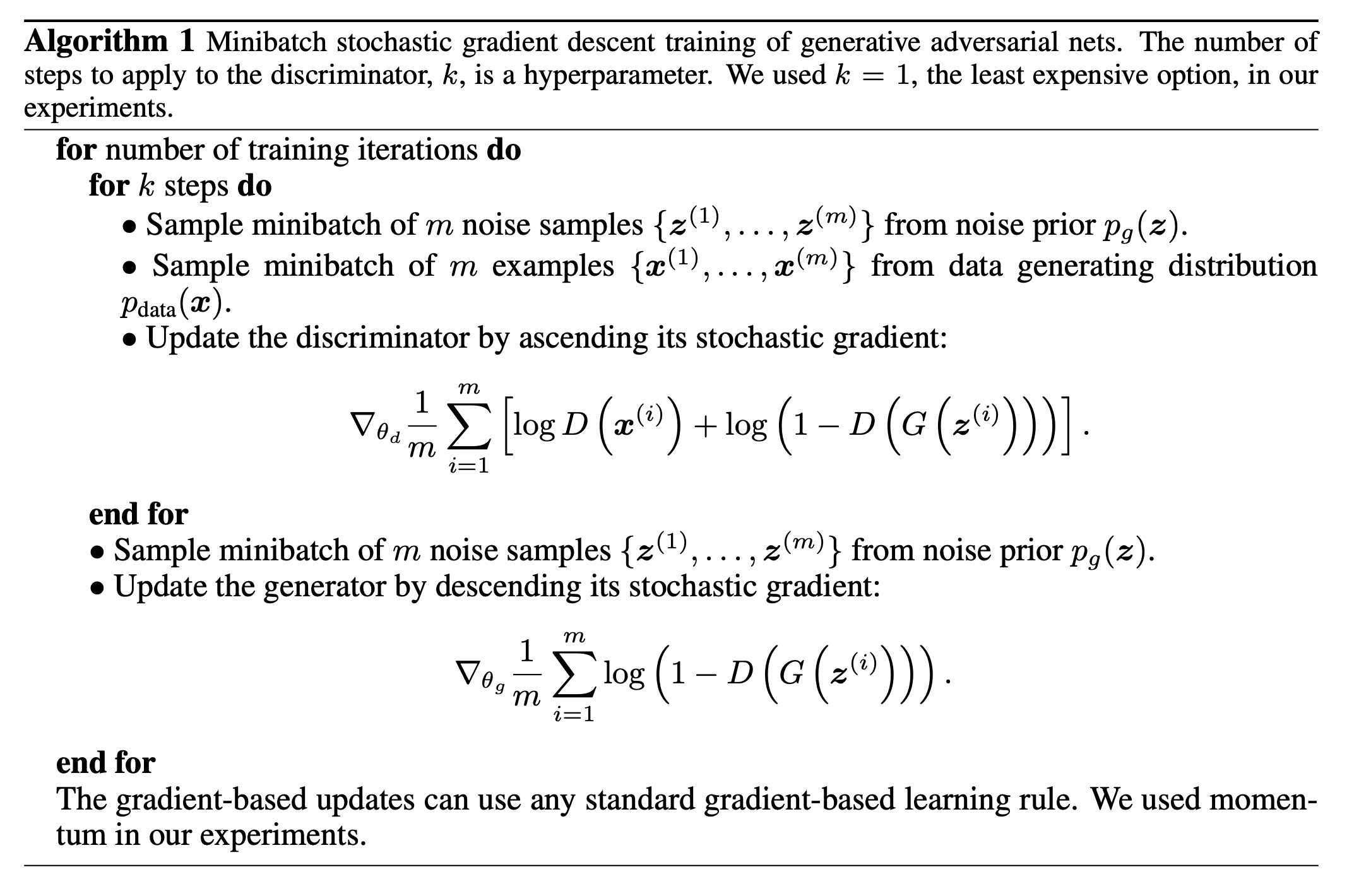 Minibatches of size \(m\) are used to train both the discriminator and the generator. There is an option to carry out \(k\) discriminator training iterations for every training step of the generator, however (more) recent empirical evidence generally shows that there isn’t typically a need for this.
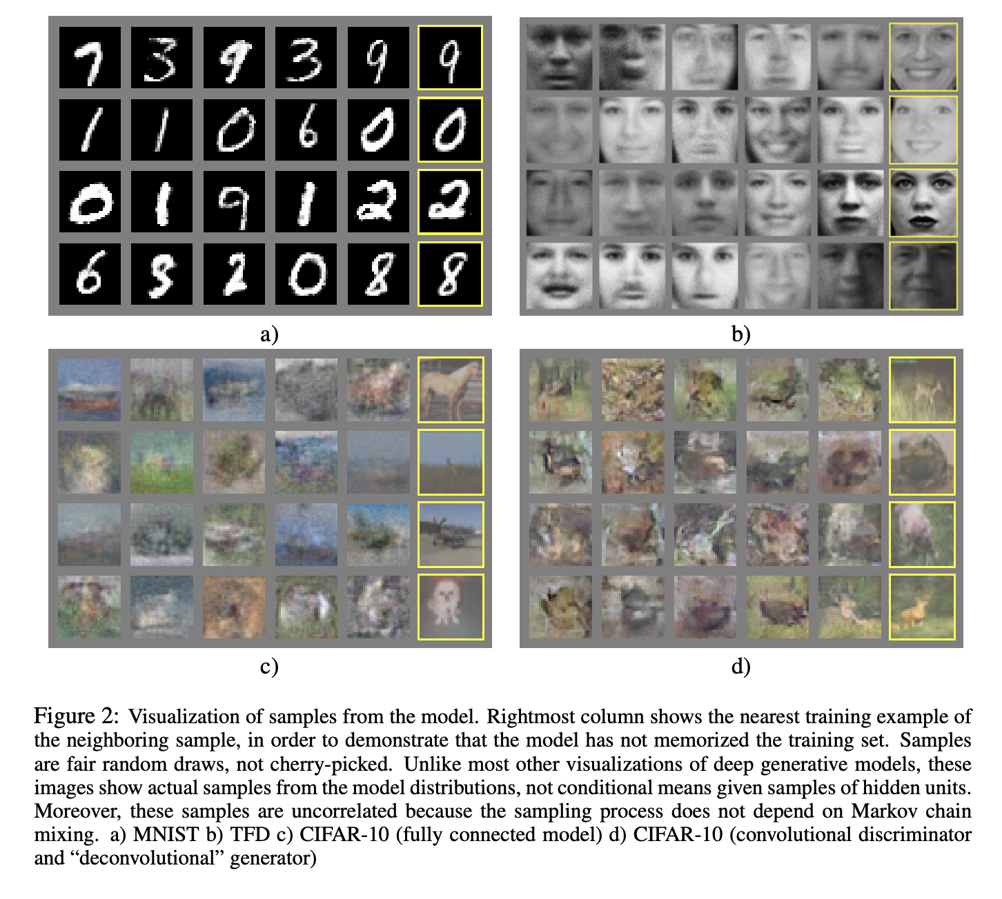
Here are the first ever published images generated by GAN experiments from the original 2014 paper.
The rightmost yellow highlighted images are from the actual dataset closest to the GAN sample left of it. They are there to ‘show’ that these GANs did not memorize the data.
GAN Lab is similar to the well know Tensor Flow Playground with which you might have played around previously. Before we dive into more examples and details, let’s play with the wonderful online GAN visualization/simulator, GAN Lab. Here is one visualization from GAN Lab:
An animation from GAN Lab live on your browser
7.3.3 We love the latent space
The use of the “latent space”, also sometimes just called a “feature vector” is a very powerful technique sometimes related to auto-encoders. More on this is in the sections below and the next unit dealing with sequence data.
Having an image represeted via the latent space is very powerful. What happens if you slightly perturb the \(Z\) in the latent space? What if you interpolate between two images?
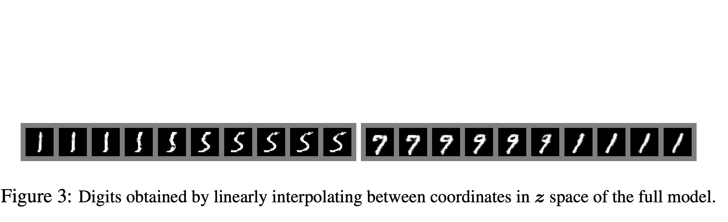
Taken from the 2014 Goodfellow et. al. paper
Lets get a feel for such perturnabtions of the latent space by playing with a very simple analogy (almost too simple). Say we have data from a univariate exponential distribution with mean \(1\).
Note that \(p(x)\) is not a probability but \(p(x) \cdot dx\) for small \(dx\) approximates the probability of falling in the region \([x,x+dx)\). The density for \(x \ge 0\) is, \[ p(x) = e^{-x}. \]
If we were to somehow have a generative model for generating \(x\), what would it be?
One general method for generating (Monte Carlo sampling) a random variable from effectively any uni-variate distribution is the inverse probability transform. Say the CDF (cumulative distribution function) of \(X\) is \(F(x)\) (and for simplicity assume it is continuous). The inverse CDF is denoted \(F^{(-1)}(u)\) (it is the quantile function). If we take a uniform \([0,1]\) random variable, \(U\), then the random variable \(F^{-1}(U)\) will be distributed with CDF \(F(\cdot)\).
In the case of exponential, \[ F(x) = \begin{cases} 0 & x < 0, \\ 1- e^{-x} & x \ge 0. \end{cases} \] Hence we can show that the inverse function is Just observe that \(F^{-1}\big(F(x)\big) = x\). \[ F^{(-1)}(u) = - \log(1-u). \]
So now we can call \(U \in [0,1]\) our latent random variable. For every \(U\) we have an \(X\) which we generate via,
In this example the distribution of \(-\log(1-U)\) is the same as that of \(-\log U\), so for simplicity we can use the latter.
\[ X = - \log U. \]
Hence the model \(-\log(\cdot)\) is a ‘generative’ model for generating samples from \(p(\cdot)\) (this is a very simple example!!!).
Now if we perturb the value \(U\) in the latent space slightly then \(X\) will be perturbed slightly also! The same happens with the images perturbations on higher dimensional latent spaces as well, it is simply that the latent variable \(Z\) is a vector and the generative model \(G(\cdot)\) is (much more) complicated than our \(-\log(\cdot)\) function.
7.4 A tour of GAN evolution
Since the (quite recent) original 2014 GAN paper there has been huge progress on GANs, here is a very partial quick tour of some advances. See also the GAN ZOO which presents links to dozens of key GAN papers - an evolving list.
7.4.1 Conditional GAN
The original GAN was generative with respect to \((X)\) with CGAN we also consider the labels \(Y\).
2014: Conditional Generative Adversarial Nets by Mehdi Mirza and Simon Osindero.
\[ \min _{G} \max _{D} V(D, G)=\mathbb{E}_{\boldsymbol{x} \sim p_{\text {data }}(\boldsymbol{x})}[\log D(\boldsymbol{x} \mid \boldsymbol{y})]+\mathbb{E}_{\boldsymbol{z} \sim p_{z}(\boldsymbol{z})}[\log (1-D(G(\boldsymbol{z} \mid \boldsymbol{y})))] \]
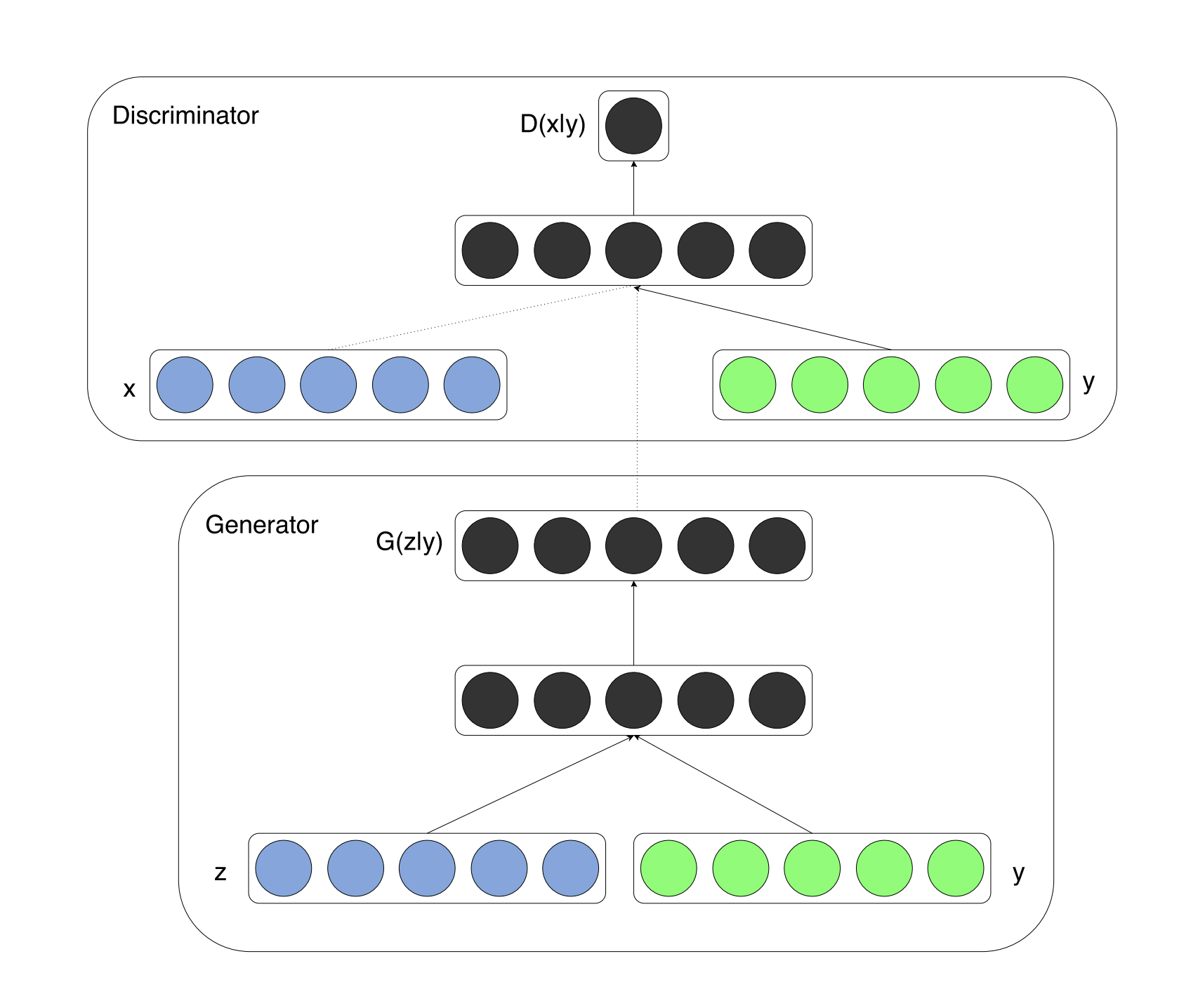
Taken from the 2014 CGAN paper
Here is conditional GAN used for MNIST:
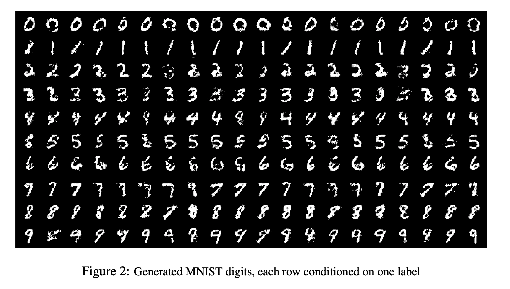
Taken from the 2014 CGAN paper
7.4.2 Convolutional GAN
The original GAN used fully connected networks. But it is very sensible to use convolutional networks
2016: Unsupervised representation learning with deep convolutional generative adversarial networks, by Alec Radford, Luke Metz, and Soumit Chintala.
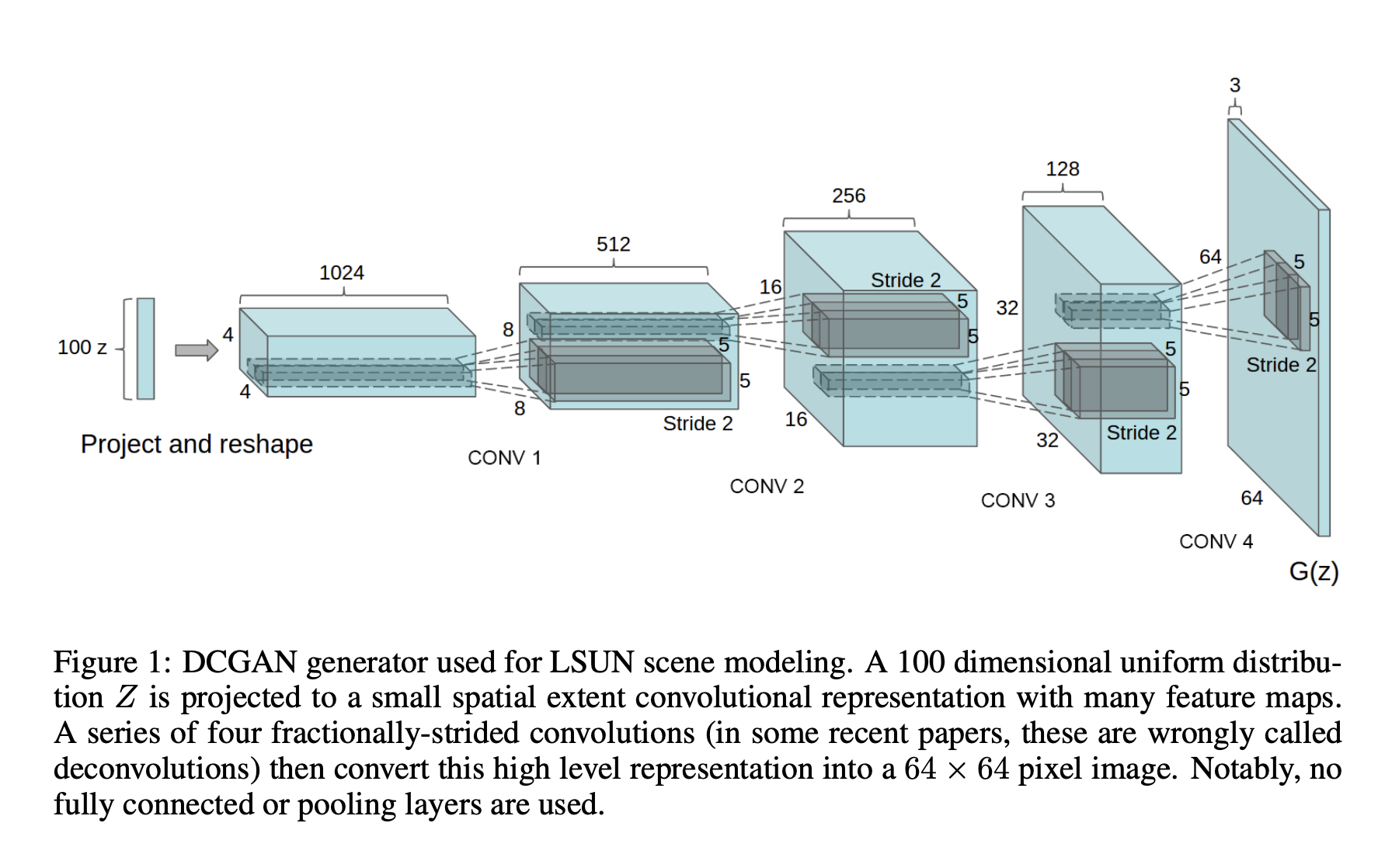
Taken from 2016 DCGAN paper
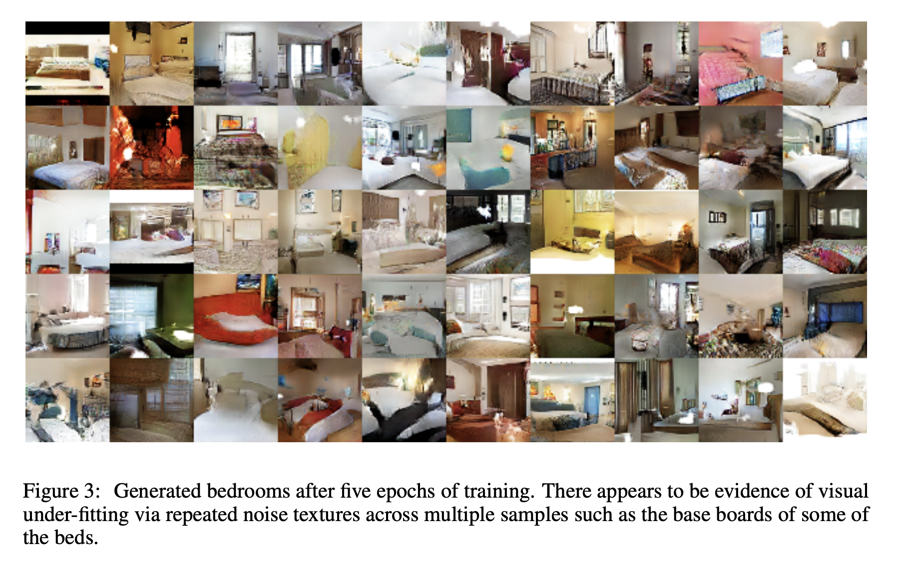
Taken from 2016 DCGAN paper
This hints that there may be meaningful semantics in the latent space.
The strength of the latent space is further demonstrated.
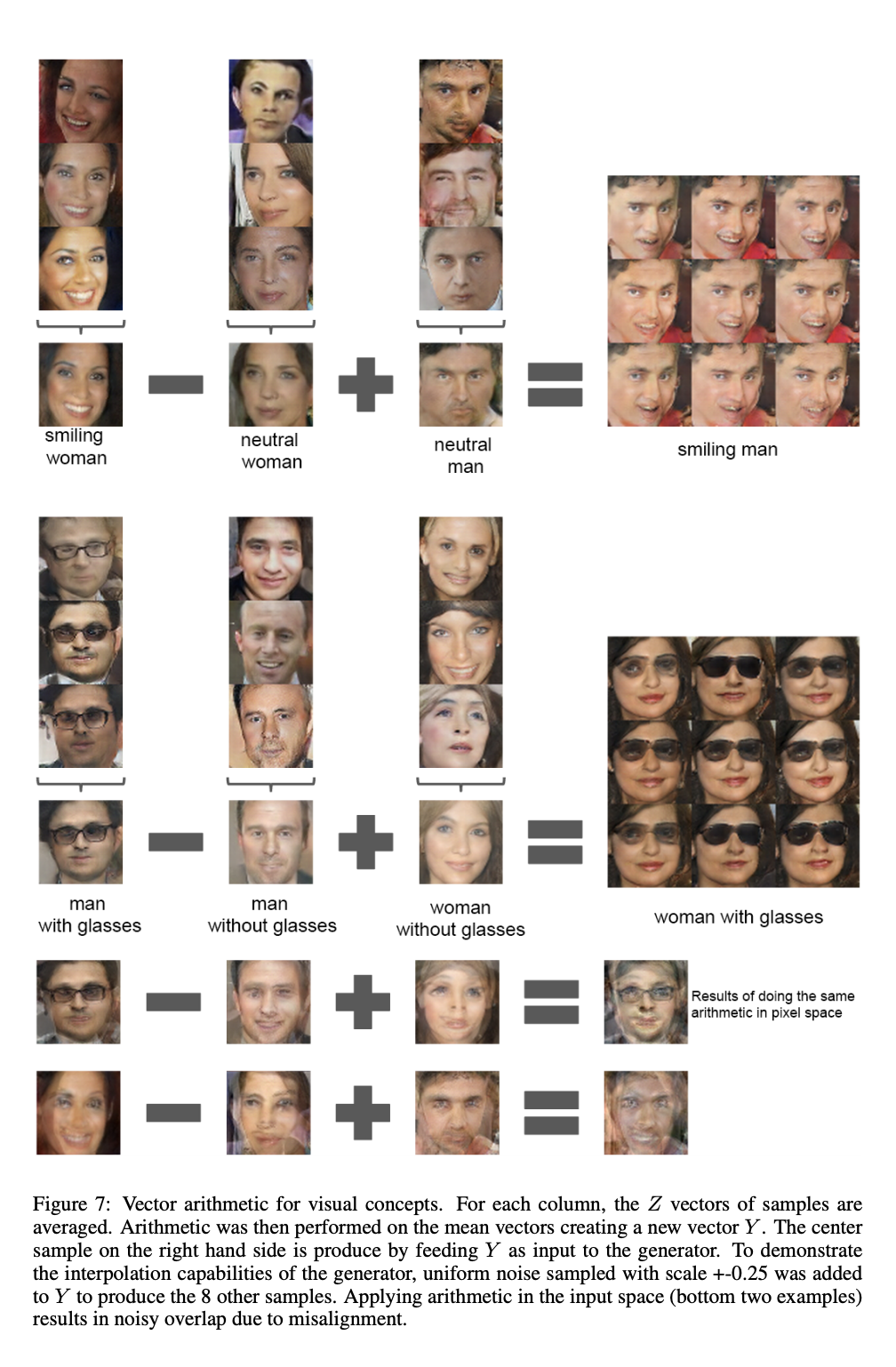
Taken from 2016 DCGAN paper
7.4.3 Large Scale GAN
It took a while to generate ‘ImageNet like’ (quality) images. It is now doable. Note that this 2018 work relies on a combination of large and well-managed compute, and several other mathematical advances along the way.
2018: Large scale GAN training for high fidelity natural image synthesis by Andrew Brock, Jeff Donahue, and Karen Simonyan.
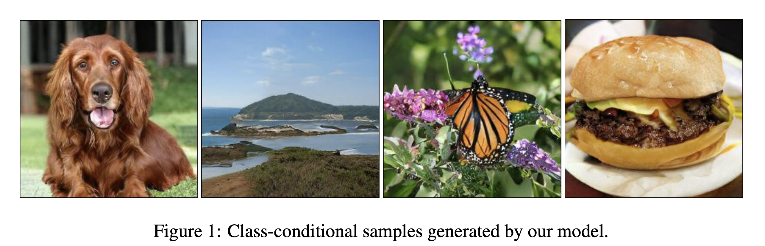
Taken from the 2018 Large Scale GAN paper
Note that in ImageNet there are about 100 dog classes and only one tennis ball class…
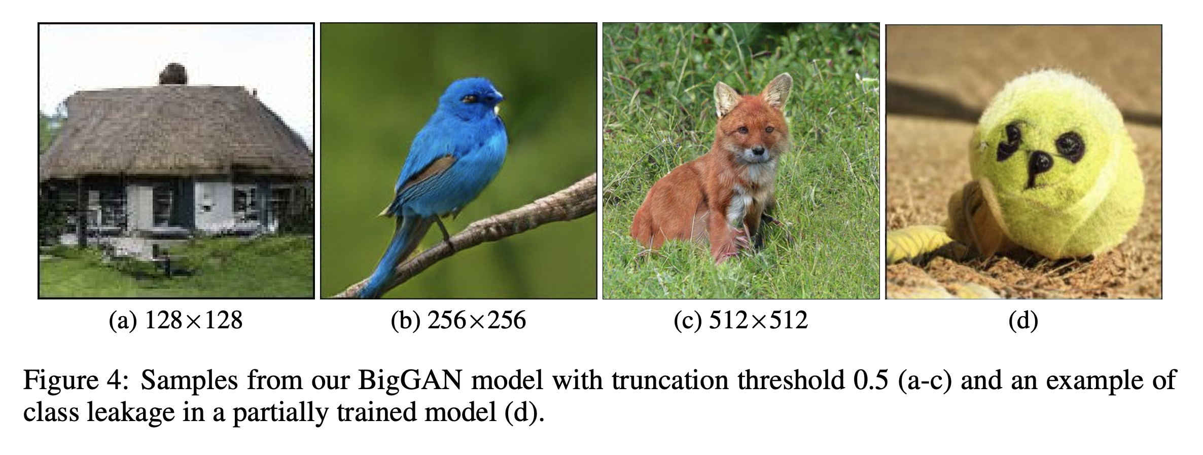
Taken from the 2018 Large Scale GAN paper
7.4.4 Style GAN
See the video at the top of this unit.
2019: A style-based generator architecture for generative adversarial networks by Tero Karras, Samuli Laine and Timo Aila.
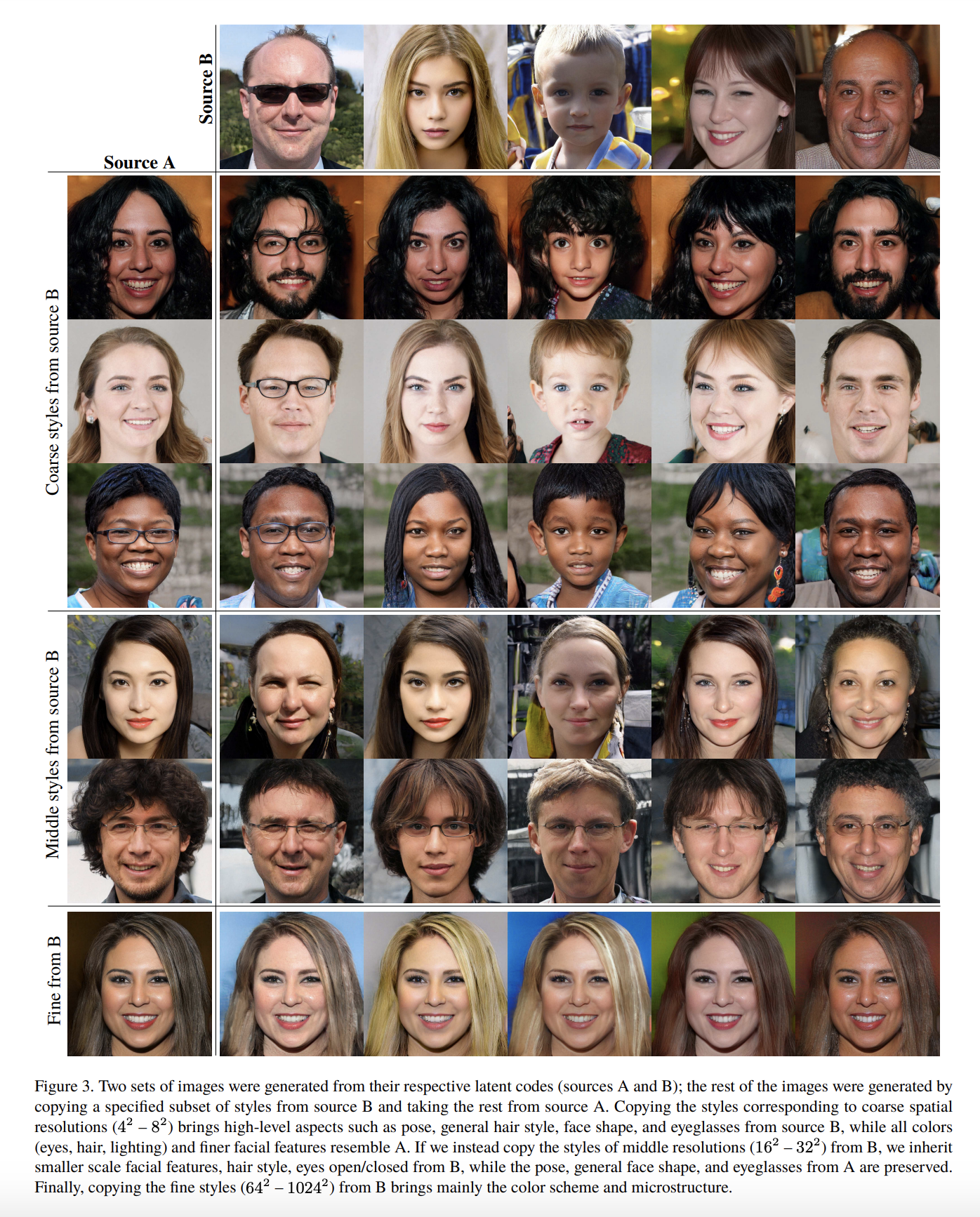
Taken from the 2019 Style GAN paper
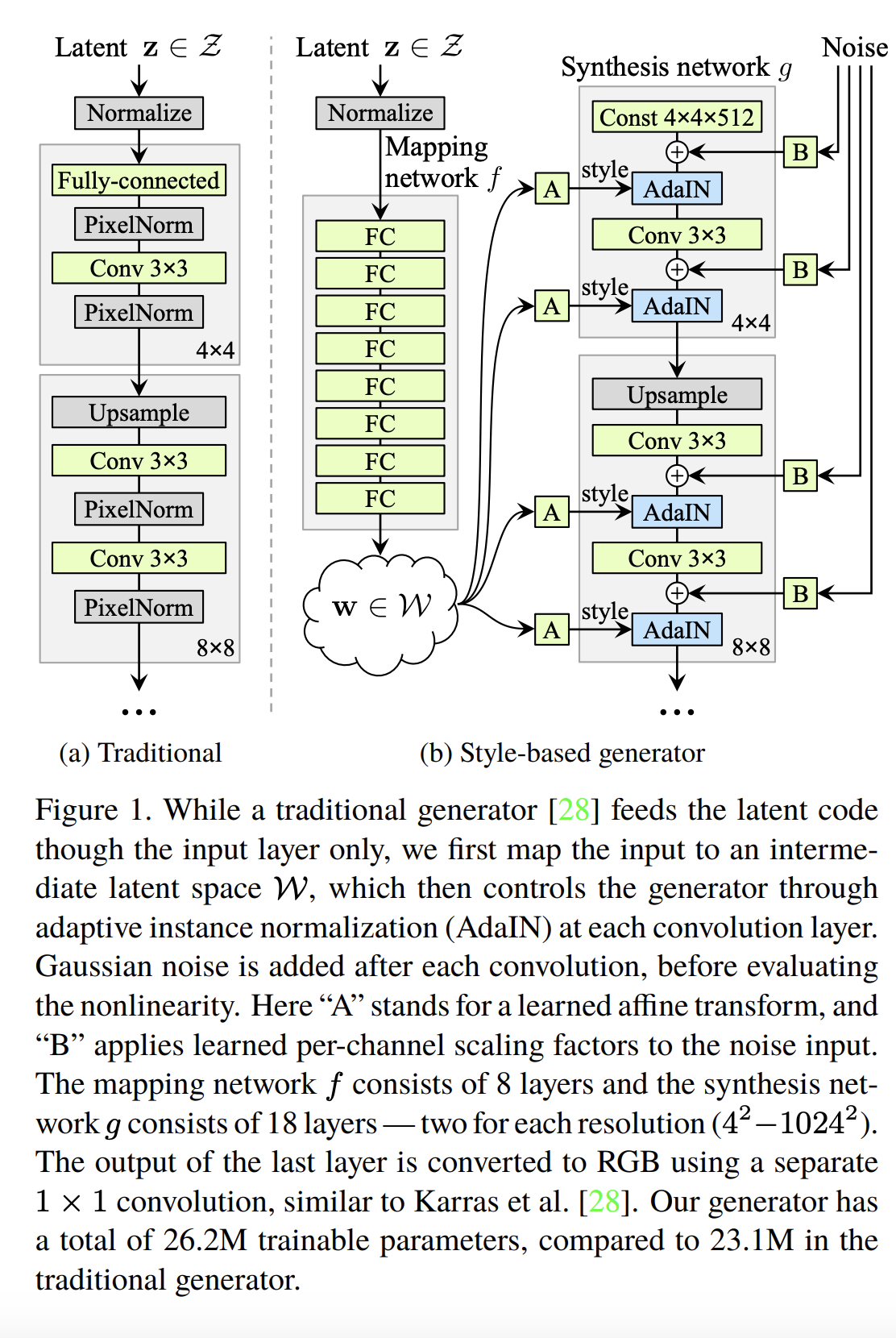
Taken from the 2019 Style GAN paper
7.5 More GAN details
Let’s dive into further mathematical details.
Observe first that if \(p=q\) then \(D_{KL}(p||q) = 0\). Observe further that KL is asymmetric: In general \(D_{KL}(p||q) \neq D_{KL}(q||p)\). First review the KL (Kullback-Leibler) divergence. It considers two probability distributions \(p\) and \(q\) and measures “how one diverges from the other”:
\[ D_{KL}(p||q) = \int_x p(x) \log \frac{p(x)}{q(x)} \, dx. \]
The Jensen-Shanon (JS) divergence also measures similarity between two probability distributions. It is defined as follows:
\[ D_{JS}(p||q) = \frac{1}{2} \Big(D_{KL}(p || r) + D_{KL}(q ||r) \Big), \qquad \text{where} \qquad r = \frac{p+q}{2}. \]
Here are some properties of the JS divergence:
- It is symmetric in \(p\) and \(q\).
- It is bounded:
Note that if we use log base \(2\) then it is bounded between in \([0,1]\).
\[ 0 \le D_{JS}(p||q) \le \log 2. \]
It is sometimes called the information radius or total divergence to the average.
It can be used to make a proper metric (its square root is a metric).
7.5.1 Vanilla GAN minimizes the JS Divergence
We denote \(p_g(x)\) as the distribution of samples generated by \(G(\cdot)\). Let’s first observe that for fixed \(G\), the optimal discriminator \(D\) is, \[ D^*(x) = \frac{p_{\text{data}(x)}}{p_{\text{data}(x)} + p_g(x)}, \] where \(p_g(\cdot)\) is the density of \(G(z)\) based on the density \(p_z(\cdot)\) of the latent space.
To see this observe that for fixed \(G\), the objective of \(D\) is to maximize,
\[ \begin{array}{rcl} V(G, D) &=&\int_{\boldsymbol{x}} p_{\text {data }}(\boldsymbol{x}) \log (D(\boldsymbol{x})) d x+\int_{z} p_{\boldsymbol{z}}(\boldsymbol{z}) \log (1-D(G(\boldsymbol{z}))) d z \\ &=&\int_{\boldsymbol{x}} p_{\text {data }}(\boldsymbol{x}) \log (D(\boldsymbol{x}))+p_{g}(\boldsymbol{x}) \log (1-D(\boldsymbol{x})) d x. \end{array} \]
Now consider the function \(f(y) = a \log (y)+b \log (1-y)\). It achieves it’s maximum at, \[ y = \frac{a}{a+b}, \] so for any fixed \(x\), \[\begin{align*} & \int_{\boldsymbol{x}} p_{\text {data }}(\boldsymbol{x}) \log (D(\boldsymbol{x}))+p_{g}(\boldsymbol{x}) \log (1-D(\boldsymbol{x})) d x \\ & \le \int_{\boldsymbol{x}} p_{\text {data }}(\boldsymbol{x}) \log (\frac{p_{\text{data}(x)}}{p_{\text{data}(x)} + p_g(x)})+p_{g}(\boldsymbol{x}) \log (1-\frac{p_{\text{data}(x)}}{p_{\text{data}(x)} + p_g(x)}) d x\\ &:= C(G) \end{align*}\]
Observe that, \[ C(G) = -\log 4 + 2 D_{JS}(p_{\text{data}}||p_{g}) \]
See proof details in the original 2014 GAN paper. Now the generator wants to minimize \(C(G)\). It can be shown that it is achieved when \(p_g(\cdot) = p_{\text{data}}(\cdot)\) at which point \(C(G) = - 2 \log 2\).
Hence the theoretical “solution” of a GAN has \(p_g = p_{\text{data}}\) in which case the value \(V(G,D)\) is \(-\log4 \approx -1.3862\).
7.5.2 Mode Collapse
While the game has a theoretical equilibrium, in practice we may sometimes not converge to \(p_g = p_{\text{data}}\). This is sometimes called mode colapse. There are several possible reasons for this:
- The equilibrium is not necessarily unique.
- The fact an equilibrium exists does not necessarily mean that an iterative approach will converge to it.
- The equilibrium is only guaranteed to exist for fully expressive models where the network of \(G(\cdot)\) has “enough parameters” to specify any distribution (specifically the distribution \(p_{\text{data}}\)).
- Distributions with non-overlapping support: In cases where in the training process there is non-overlapping or little joint support between \(p_g\) and \(p_{\text{data}}\) then learning ‘gets stuck’.
We focus on the last bullet point by modifing the value function, as described below.
7.6 Modification of Loss/Objective Function
A general survey papers whcih presents several GAN loss functions and compares them empirically is the following:
2018: Are GANs Created Equal? A Large-Scale Study by Mario Lucic, Karol Kurach, Marcin Michalski, Sylvain Gelly and Olivier Bousquet.
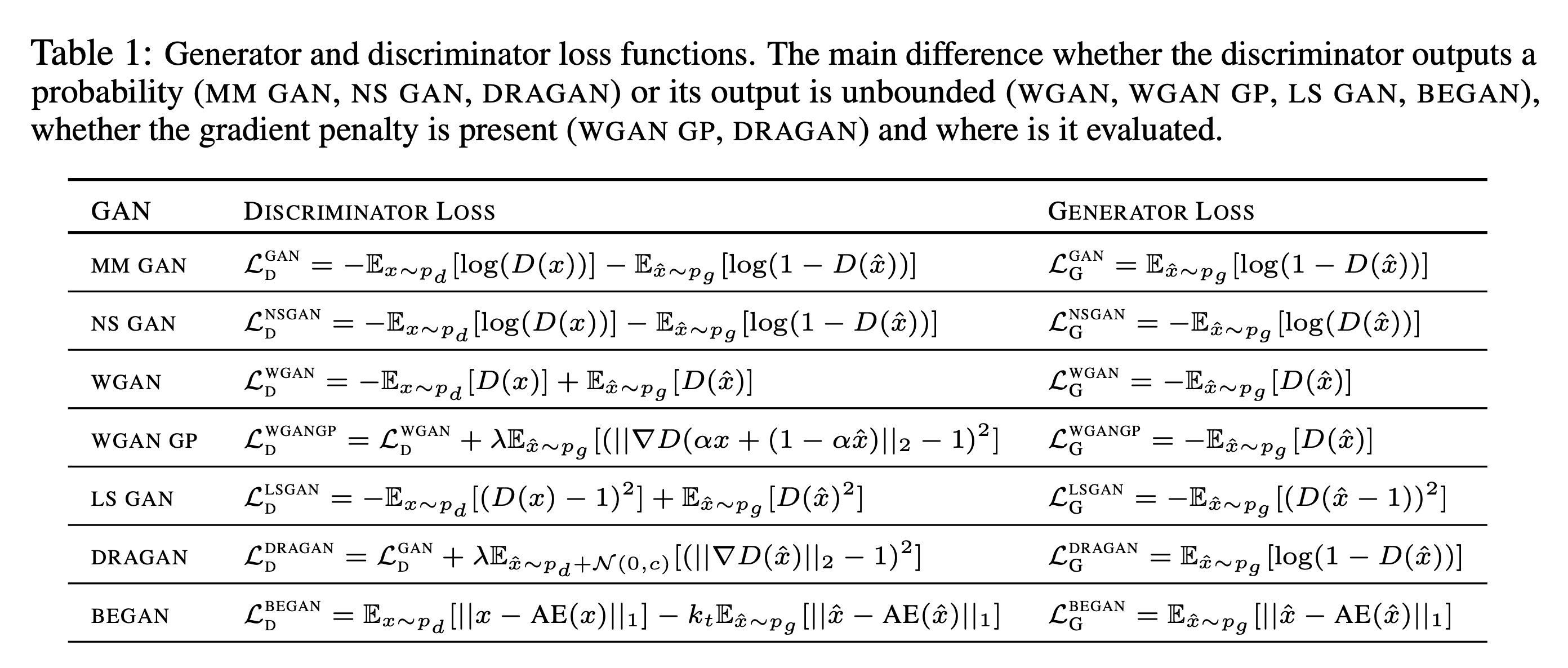
Taken from the 2018 “GANs created Equal?” paper
We will focus on the Wasserstein GAN initially presented here:
- 2017: Wasserstein generative adversarial networks by Martin Arjovsky, Soumith Chintala and Leon Bottou.
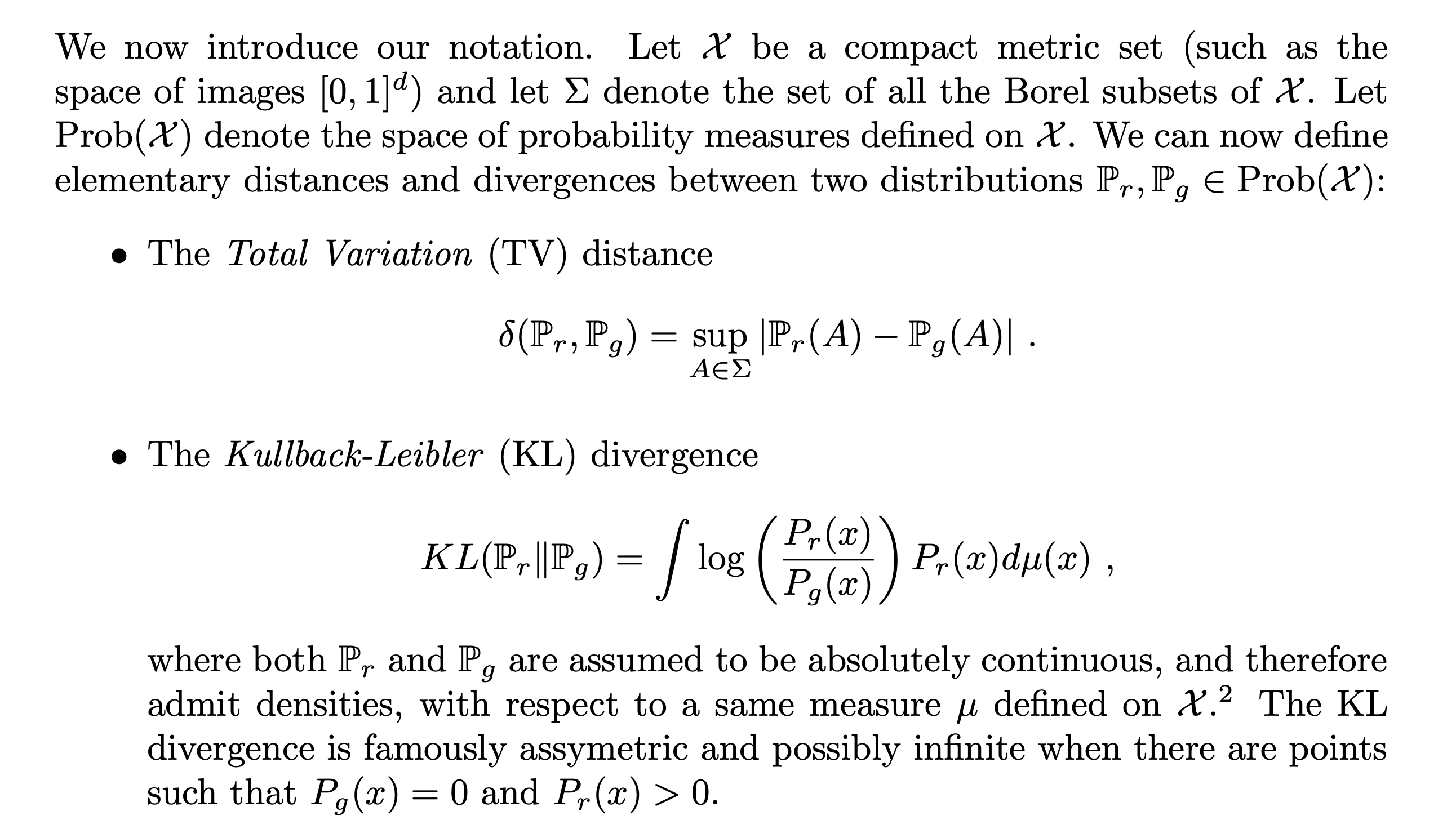
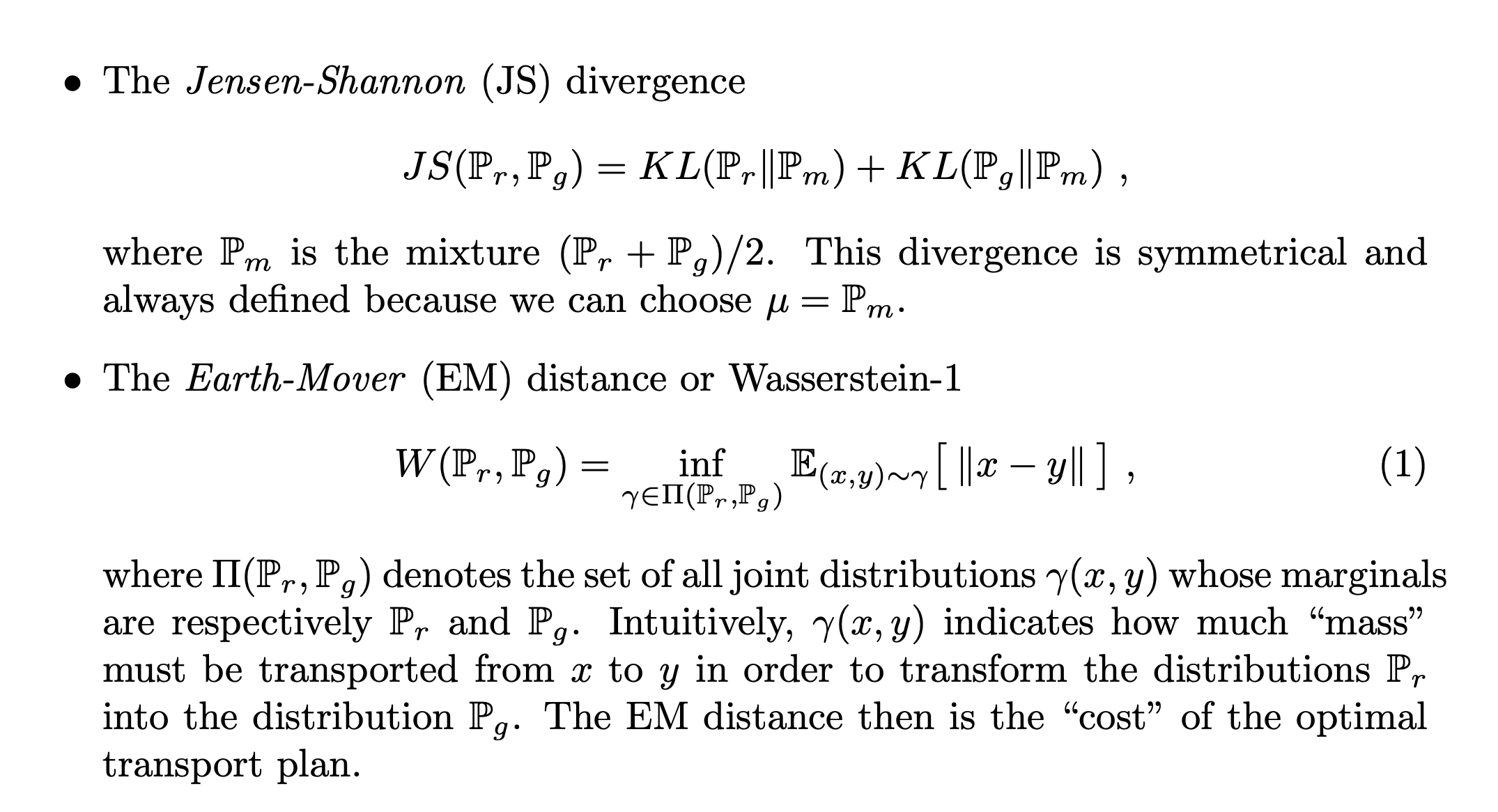
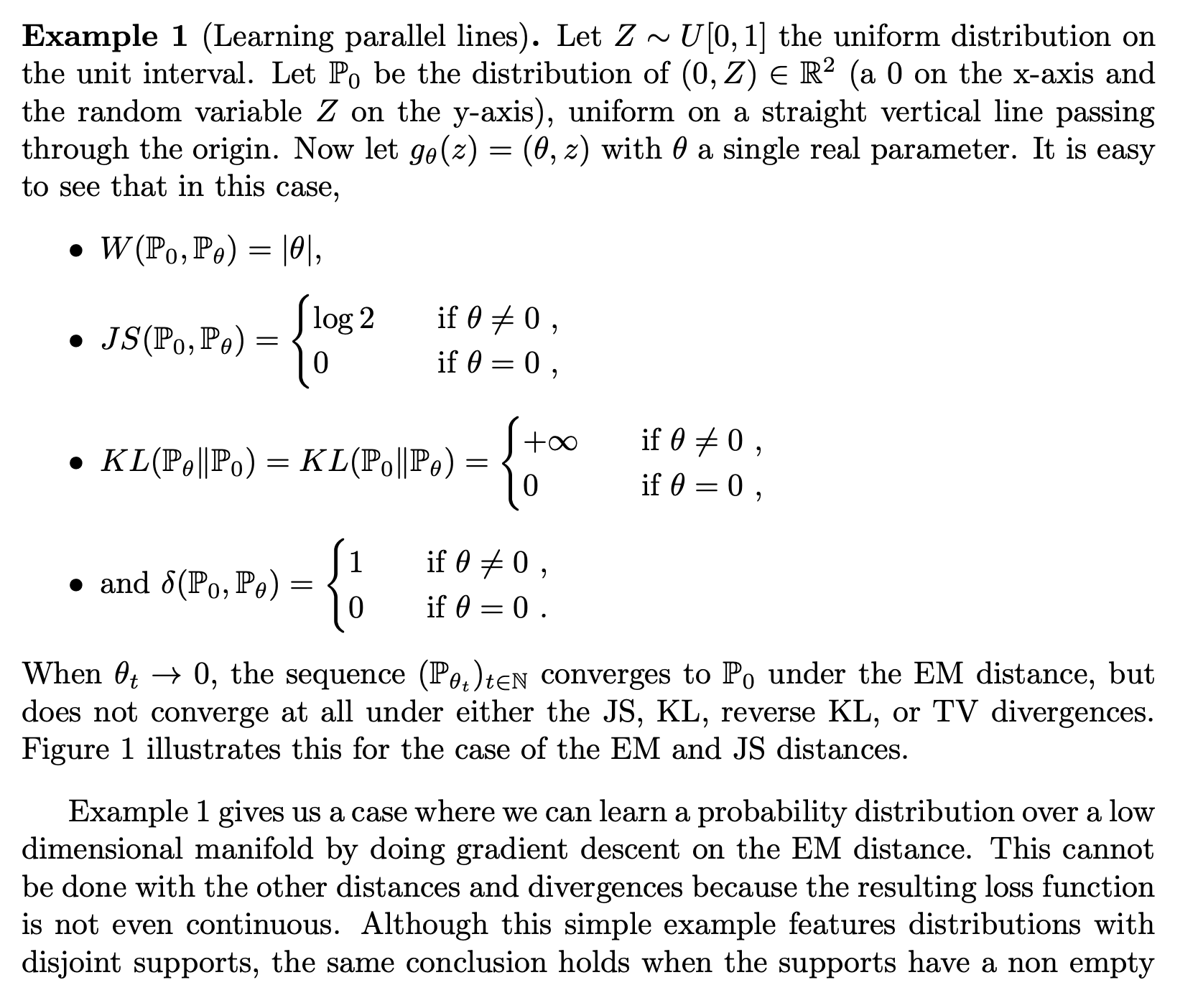
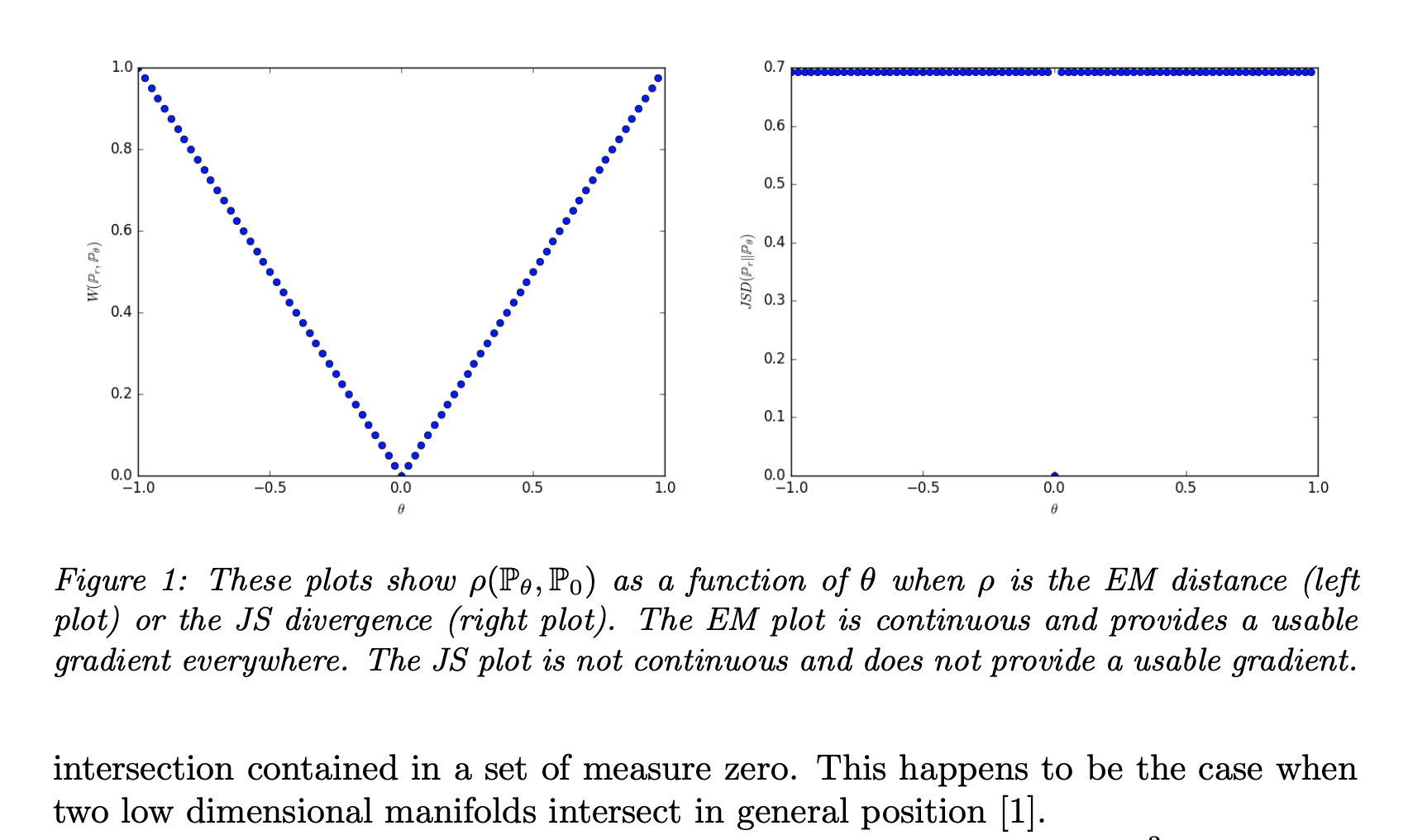
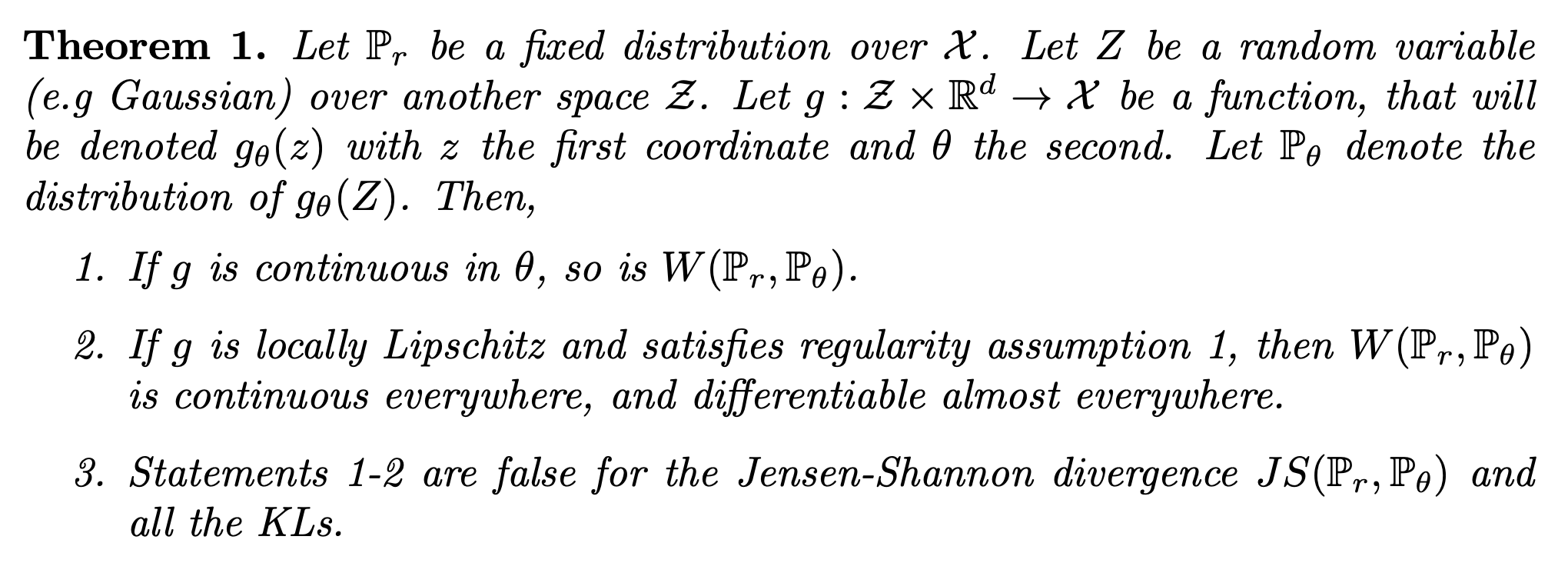
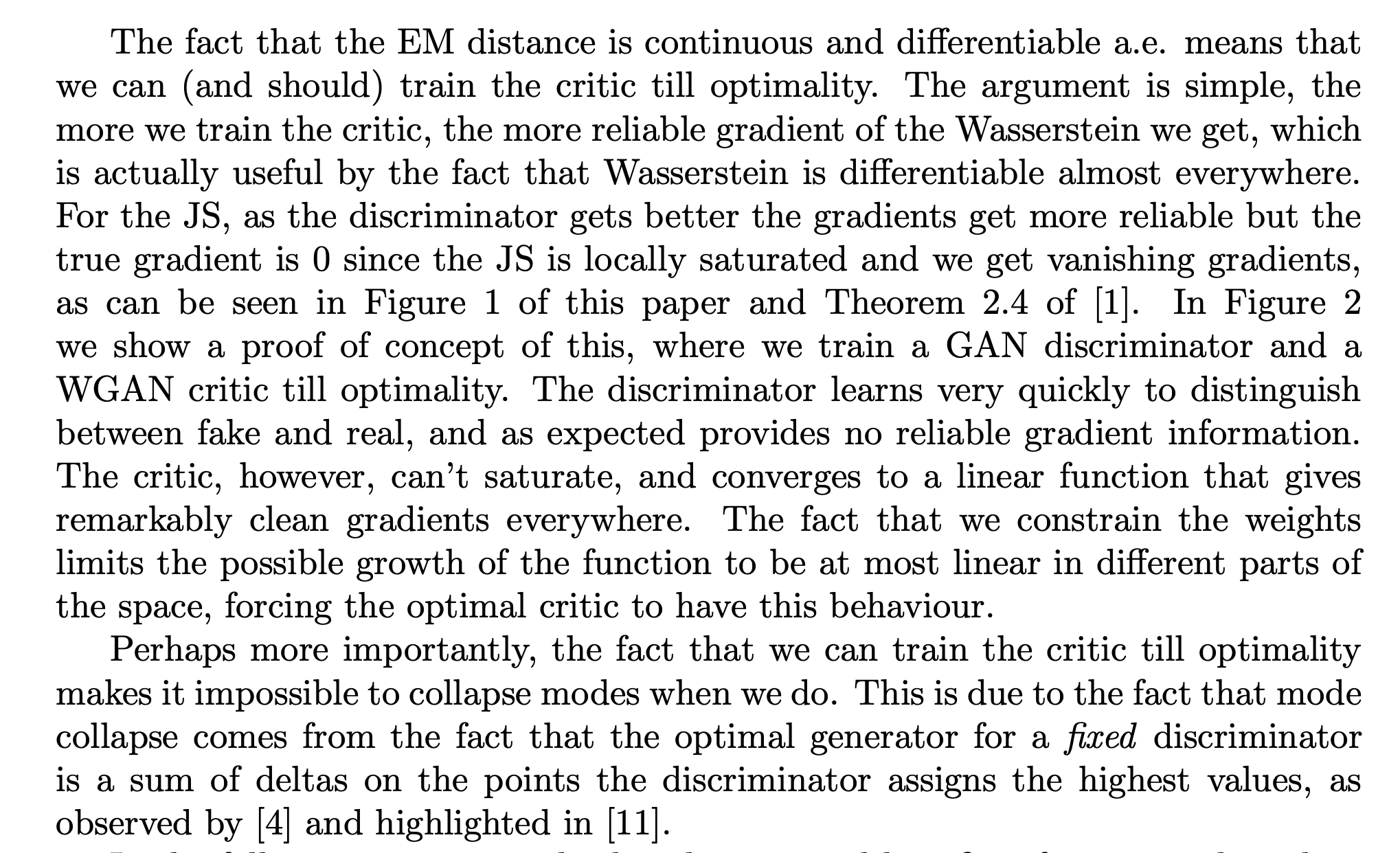
Below are key snippets from the 2017 WGAN paper where some theoretical justification for using the Wasserstein GAN are presented.
7.6.1 Some basis for the Earth Mover (or Wasserstein) distance
7.6.2 The WGAN algorithm
The infimum in the Wasserstein distance,
\[ W\left(\mathbb{P}_{r}, \mathbb{P}_{g}\right)=\inf _{\gamma \in \Pi\left(\mathbb{P}_{r}, \mathbb{P}_{g}\right)} \mathbb{E}_{(x, y) \sim \gamma}[\|x-y\|] \]
is highly non-attainable. However, the Kantorovich-Rubinstein duality tells us that,
\[ W\left(\mathbb{P}_{r}, \mathbb{P}_{\theta}\right)=\sup _{\|f\|_{L} \leq 1} \mathbb{E}_{x \sim \mathbb{P}_{r}}[f(x)]-\mathbb{E}_{x \sim \mathbb{P}_{\theta}}[f(x)], \] where the supremum is over all \(1\)-Lipschitz functions, i.e., \[ ||f(x) - f(y)|| \le 1 \cdot ||x-y|| \]
It still isn’t easy to compute this metric, but it inspires using the discrimentator \(D(\cdot)\) as \(f(\cdot)\). Note that now the discriminator is not longer a binary classifier. Hence the WGAN objective is
\[ \min_G \max_{D: ||D||_L \le 1} \mathbb{E}_{x \sim \mathbb{p}_{\text{data}}}[D(x)]-\mathbb{E}_{z \sim \mathbb{p}_{z}}[D(G(x))], \]
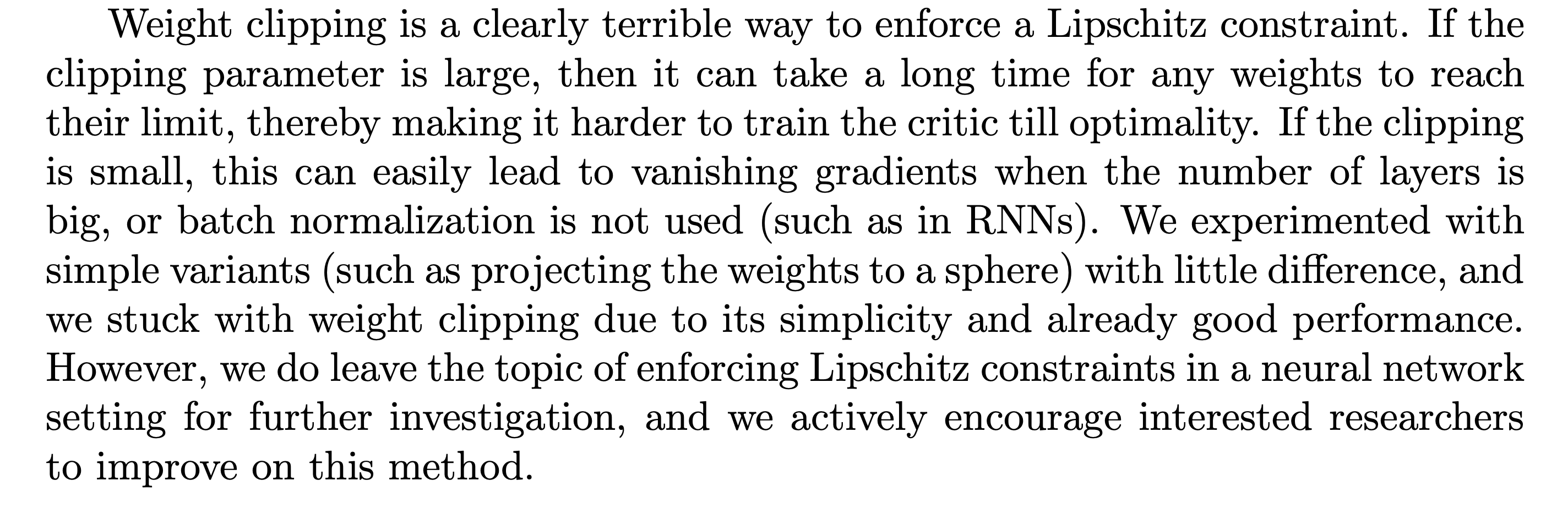
There is the problem of how to deal with the constraint, \(: ||D||_L \le 1\). A crude (first) way to do this is via clipping. Here is the algorithm from the WGAN paper
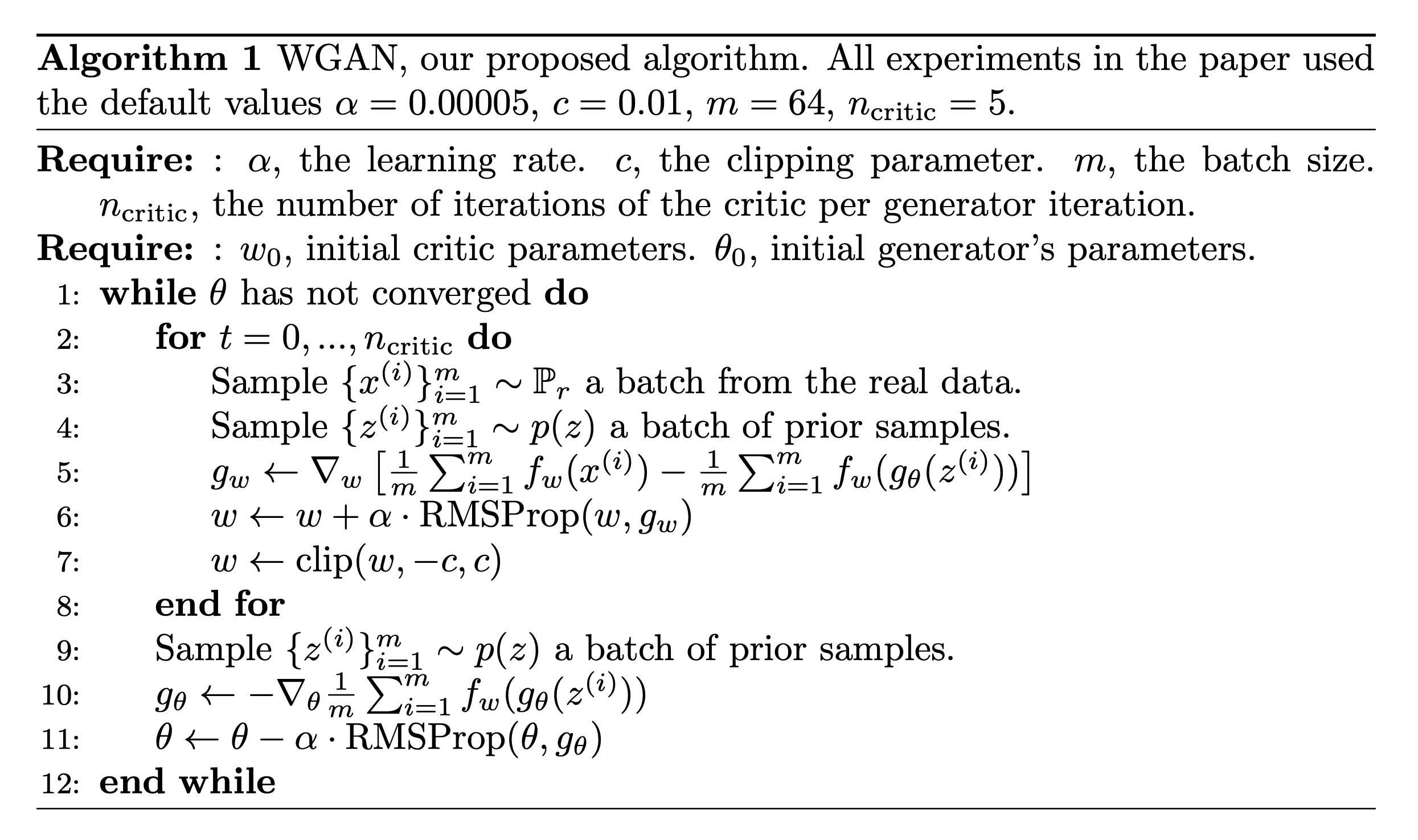
Taken from the WGAN paper
Here are comments also taken from the WGAN paper:
7.7 Quality Measures
It isn’t obvious how to evaluate the performance of a GAN. Here are some current methods:
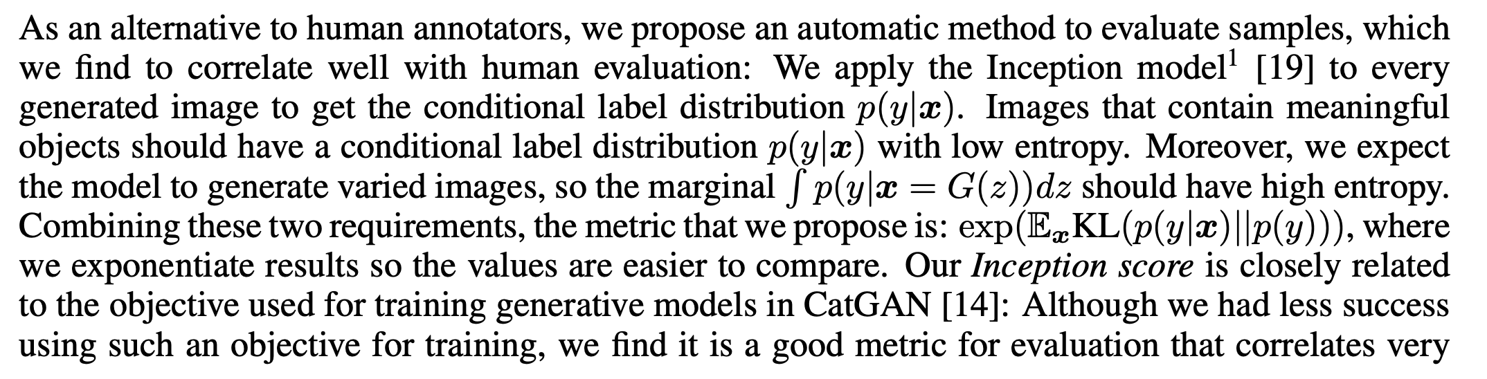
- Inception Score:
2016: Improved techniques for training gans by Tim Salimans, Ian Goodfellow, Wojciech Zaremba, Vicki Cheung, Alec Radford, and Xi Chen.
Taken from that paper:
- Fréchet Inception Distance (FID):
For a definition see:
2017: Gans trained by a two time-scale update rule converge to a local nash equilibrium by Martin Heusel, Hubert Ramsauer, Thomas Unterthiner, Bernhard Nessler, and Sepp Hochreiter.
7.8 Applications
See for example this blog post. These are some of the applications of GANs:
- Generate Examples for Image Datasets (data augmentation)
- Generate Realistic Photographs
- Image-to-Image Translation
- Text-to-Image Translation
- Photos to Emojis
- Photograph Editing
- Face Aging
- Photo Blending
- Super Resolution
- Photo Inpainting
- Video Prediction
- 3D Object Generation
- Semi-supervised learning
This is still an evolving field. This (quite recent) talk by Ian Goodfellow presents an overview of GANs and the evolving applications:
However we must also acknowledge that there is significant danger with GAN technology, specifically dealing with DeepFakes. Deep fakes pose not only political danger but also private danger. See for example this video:
they are more resilient to vanishing gradients
Page built: 2021-03-04 using R version 4.0.3 (2020-10-10)