See the latest book content here.
3 Optimization Algorithms
In this chapter we focus on general approach to optimization for multivariate functions. In the previous chapter, we have seen three different variants of gradient descent methods, namely, batch gradient descent, stochastic gradient descent, and mini-batch gradient descent. One of these methods is chosen depending on the amount of data and a trade-off between the accuracy of the parameter estimation and the amount time it takes to perform the estimation. We have noted earlier that the mini-batch gradient descent strikes a balance between the other two methods and hence commonly used in practice. However, this method comes with few challenges that need to be addressed. We also focus on these issues in this chapter.
Learning outcomes from this chapter:
Several first-order optimization methods
Basic second-order optimization methods
This chapter closely follows chapters 4 and 5 of (Kochenderfer and Wheeler 2019). There are many interesting textbooks on optimization, including (Boyd and Vandenberghe 2004), (Sundaram 1996), and (Nesterov 2004),
3.1 Preliminaries
In this section, we establish some preliminaries that are necessary for understanding the methods discussed later.
3.1.1 Directional Derivative
Consider an \(n\)-dimensional multivariate function \(f : \Theta \to \mathbb R\) over a feasible set \(\Theta \subseteq \mathbb R^n\).
The gradient of \(f\) at \(\theta\), when exists, is given by \[\nabla f(\theta) = \left[\frac{\partial f(\theta)}{\partial x_1}, \dots, \frac{\partial f(\theta)}{\partial x_n} \right],\] which is a vector capturing the local slope of the function \(f\) at \(\theta\).
The directional derivative \(\nabla_{\mathbf s} f(\theta)\) of \(f\) at \(\theta\) in the direction of \(\mathbf s = [s_1, \dots, s_n]\) is defined by \[\nabla_{\mathbf s} f(\theta) = \lim_{h \to 0} \frac{f(\theta + h \mathbf s) - f(\theta)}{h}.\]
Note that \(\frac{\partial f(\theta)}{\partial x_i}\) is the directional derivative at \(\theta\) in the direction of the vector \(\mathbf e_i\) consists of \(1\) at the \(i\)-th location and zeros everywhere else. This simply follows from the observation that \[\nabla_{\mathbf e_i} f(\theta) = \lim_{h \to 0} \frac{f(x_1, \dots, x_i + h, \dots, x_n) - f(\theta)}{h}.\]
Thus, \(s_i\frac{\partial f(\theta)}{\partial x_i}\) is the directional derivative at \(\theta\) in the direction of the vector \(s_i\mathbf e_i\).
Together, we can conclude that the directional derivative at \(\theta\) in the direction \(\mathbf s\) is
where \(\boldsymbol{\cdot}\) denotes the dot product between vectors.
- Alternatively, we can obtain the above relation between the gradient and directional derivative by observing from the first-order approximation \(f(\theta + h \mathbf s) = f(\theta) + \nabla f(\theta) \boldsymbol{\cdot}(h\mathbf s) + O(h^2)\) that
\[ \frac{f(\theta + h \mathbf s) - f(\theta)}{h} = \mathbf s \boldsymbol{\cdot}\nabla f(\theta) + O(h).\] Now take the limit \(h \to 0\) on both the sides.
Exercise: Show that the directional derivative \(\nabla_{\mathbf s} f(\theta)\) is maximum in the direction of the gradient. That is, for all unit length vectors \(\mathbf s\), the choice \(\mathbf s = \nabla f(\theta)/\|\nabla f(\theta)\|\) maximizes \(\nabla_{\mathbf s} f(\theta)\).
Hint: The Cauchy–Schwarz inequality for vectors.
3.1.2 Python Basics
SymPy is a Python library for symbolic mathematics. We illustrate the applications of this library with some examples.
Finding derivatives: Suppose that we want to find the derivative \(\partial f/\partial t\) of the following univariate function: \[ f(t) = \exp(-t^2/2)*\sin(\pi t). \] For this, SymPy package can be used as follows:
import sympy
import numpy as np

t = sympy.Symbol('t', real=True)
f = sympy.exp(-t**2 / 2) * sympy.sin(sympy.pi*t)

dfdt = f.diff(t) # Taking derivative with respect to t

print("Output:\n f'(t) =", dfdt, "\n f'(t) =", sympy.latex(sympy.simplify(dfdt)))
## Output:
## f'(t) = -t*exp(-t**2/2)*sin(pi*t) + pi*exp(-t**2/2)*cos(pi*t)
## f'(t) = \left(- t \sin{\left(\pi t \right)} + \pi \cos{\left(\pi t \right)}\right) e^{- \frac{t^{2}}{2}}The second output is a latex expression for
\[ f'(t) = \left(- t \sin{\left(\pi t \right)} + \pi \cos{\left(\pi t \right)}\right) e^{- \frac{t^{2}}{2}}.\]
Finding gradient: Now consider the following multivariate function:
\[f(t_1, t_2) = \exp(-t_1^2/2)*\sin(\pi t_2).\]
t1, t2 = sympy.symbols('t1, t2', real=True)

f = sympy.exp(-t1**2 / 2) * sympy.sin(sympy.pi*t2)
theta = (t1, t2)
grad = [f.diff(t) for t in theta]
print("Gradient of f: \n", grad)
## Gradient of f:
## [-t1*exp(-t1**2/2)*sin(pi*t2), pi*exp(-t1**2/2)*cos(pi*t2)]Evaluating function values: Evaluating function value at a point using SymPy. Again suppose that
\[f(t_1, t_2) = \exp(-t_1^2/2)*\sin(\pi t_2),\]
and we want to evaluate the value of \(f\) at \((t_1, t_2) = (1,3/2)\). The following code does it using subs and evalf:
t1, t2 = sympy.symbols('t1, t2', real=True)

f = sympy.exp(-t1**2 / 2) * sympy.sin(sympy.pi*t2)

print("value of f(1, 3/2):", (f.subs([(t1,1), (t2,3/2)])).evalf())
## value of f(1, 3/2): -0.606530659712633Alternatively, we can use lambdify as follows:
t1, t2 = sympy.symbols('t1, t2', real=True)

f = sympy.exp(-t1**2 / 2) * sympy.sin(sympy.pi*t2)
f = sympy.lambdify((t1, t2), f)

print("value of f(1, 3/2):", f(1,3/2))
## value of f(1, 3/2): -0.6065306597126334Note: Once we have the gradient of a function, it is easy to compute its directional derivative using (3.1).
3d plot of functions: Finally, suppose that we would like make a 3d plot of Rosebrock function:
\[f(t_1, t_2) = (a - t_1)^2 + b(t_2 - t_1^2)^2.\]
The following Python code plots \(f\) for \(a = 1\) and \(b = 100\) over \([-2, 2]\times [-1, 3]\).
import matplotlib.pyplot as plt

a = 1.0
b = 100
t1, t2 = sympy.symbols('t1, t2', real=True)
f = (a - t1)**2 + b*(t2 - t1**2)**2
f = sympy.lambdify((t1, t2), f)

def fun(x, y):
    return f(x,y)

t1_range = np.arange(-2.0,2, 0.05)
t2_range = np.arange(-1.0,3.0, 0.05)

X, Y = np.meshgrid(t1_range, t2_range)

Z = fun(X, Y)


fig = plt.figure()
ax = plt.axes(projection='3d')
ax.plot_surface(X, Y, Z, rstride=1, cstride=1,
                cmap='Blues', edgecolor='none')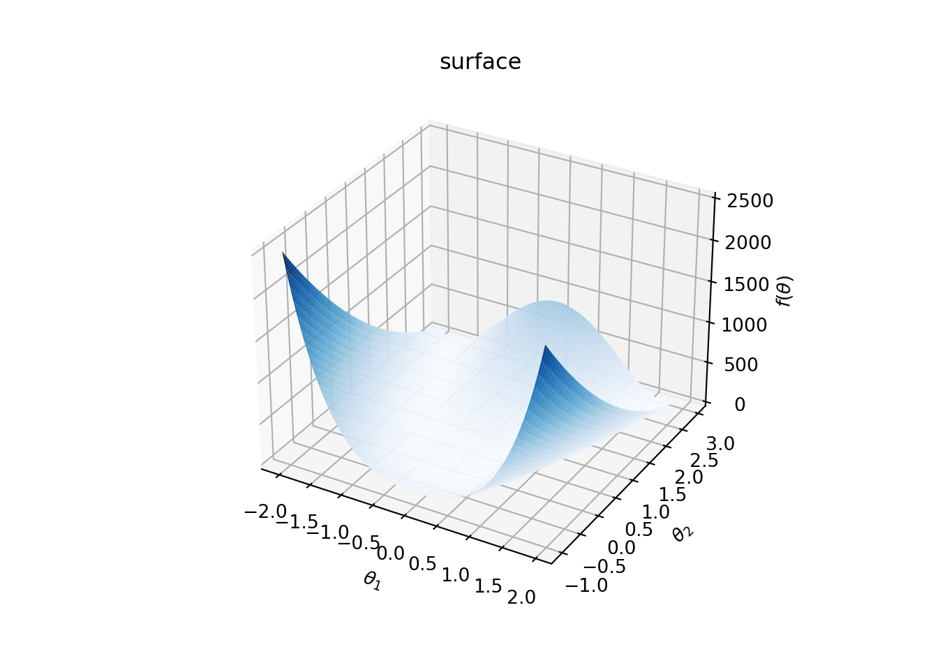
The corresponding contour plot is given by
CP = plt.contour(X, Y, Z, levels=np.exp(np.arange(-3, 7, 0.5)), cmap='Blues')
plt.clabel(CP, inline=1, fontsize=10)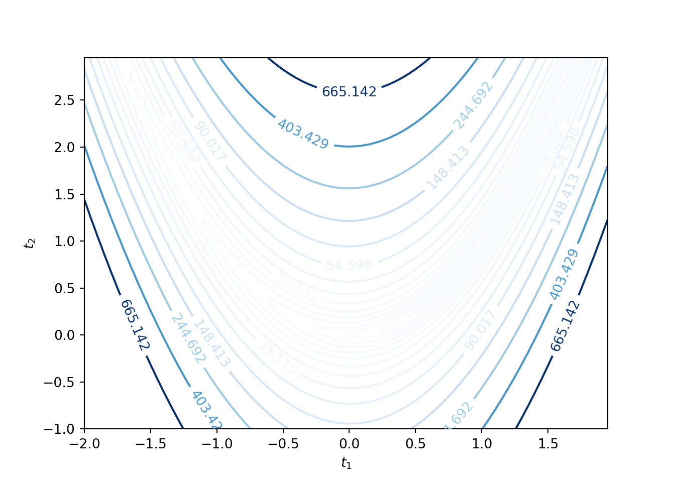
3.1.3 Local Minimum, Saddle Point, and Convexity
In this section, we look at several examples of 2-dimensional functions to understand the notions of local minimum, saddle point, and convexity.
Local Minimum: For a multivariate function \(f(\theta)\), the necessary condition for a point \(\theta\) to be at a local minumum is that the gradient \(\nabla f(\theta) = 0\) and the Hessian \[\begin{equation*} \nabla^2 f(\theta) = \begin{bmatrix} \frac{\partial^2 f}{\partial \theta_1^2 } & \frac{\partial^2 f}{\partial \theta_1 \partial \theta_2} & \cdots & \frac{\partial^2 f}{\partial \theta_1 \partial \theta_n}\\ \vdots & \vdots & \vdots & \vdots\\ \frac{\partial^2 f}{\partial \theta_n \partial \theta_1} & \frac{\partial^2 f}{\partial \theta_n \partial \theta_2} & \cdots & \frac{\partial^2 f}{\partial \theta_n^2 } \end{bmatrix} \end{equation*}\] is positive semidefinite , i.e., \(\widehat \theta \boldsymbol{\cdot}\left( \nabla^2 f(\theta) \widehat \theta\right) \geq 0\) for all \(\widehat \theta\).
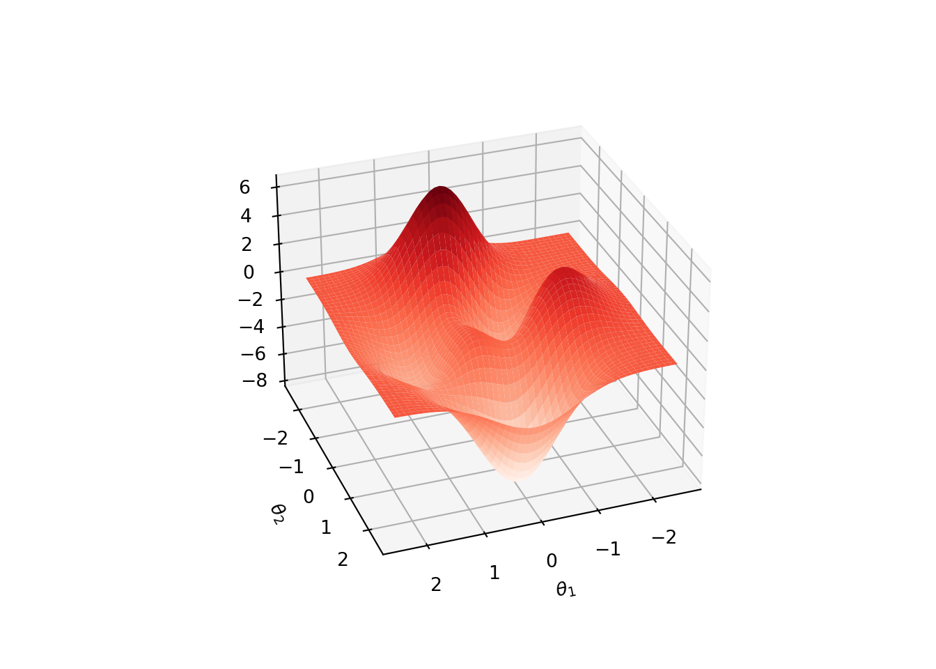
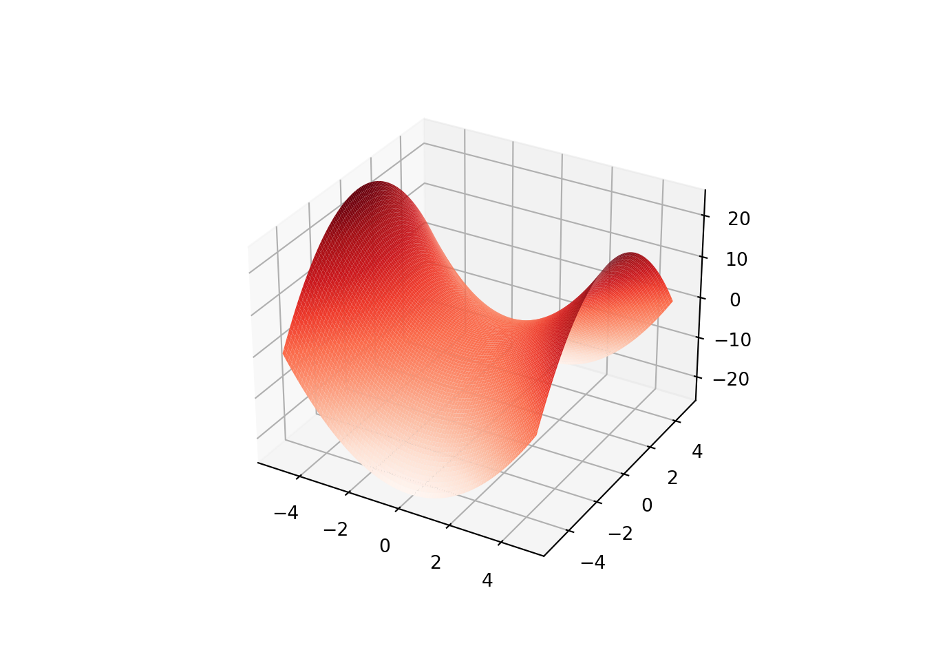
The following plot of a peaks function has multiple local minima (also mmultiple local maxima).
Convexity: A multivariate function \(f(\theta)\) is convex over a region \(\Theta \subseteq \mathbb R^n\) if the Hessian is positive semidefinite for all \(\theta \in \Theta\). Furthermore, \(f\) is strictly convex if the Hessian is poistive definite, i.e., \(\widehat \theta \boldsymbol{\cdot}\left( \nabla^2 f(\theta) \widehat \theta\right) > 0\) for all \(\widehat \theta \neq \mathbf 0\).
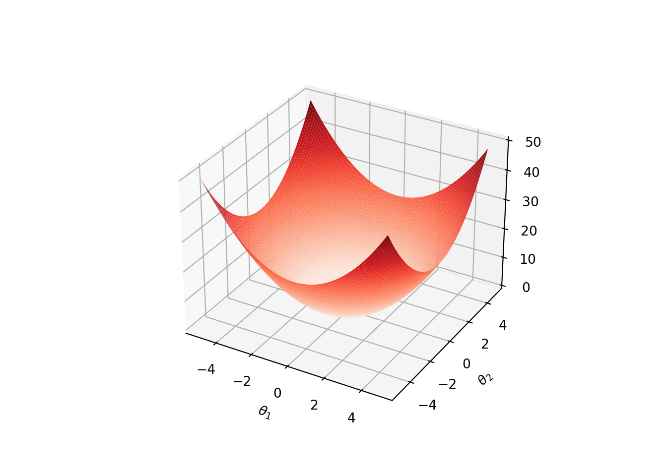
Convexity gurantees that all local minima are global minima. Strict convexity gurantees that the function has a unique global minimum. For an illustration, see the following plot of \(f(\theta) = \theta_1^2 + \theta_2^2\).
Saddle Point: A point \(\theta\) is a saddle point of \(f\) if the gradient \(\nabla f(\theta) = 0\), but \(\theta\) is not a local extrememum of \(f\). Necessary condition for a point \(\theta\) to be a saddle point is that the gradient \(\nabla f(\theta) = 0\) and the Hessian \(\nabla^2f(\theta)\) is indefinite (neither positive semidefinite nor negative definite).
For \(f(\theta) = \theta_1^2 - \theta_2^2\) plotted below, \((0,0)\) is a saddle point.
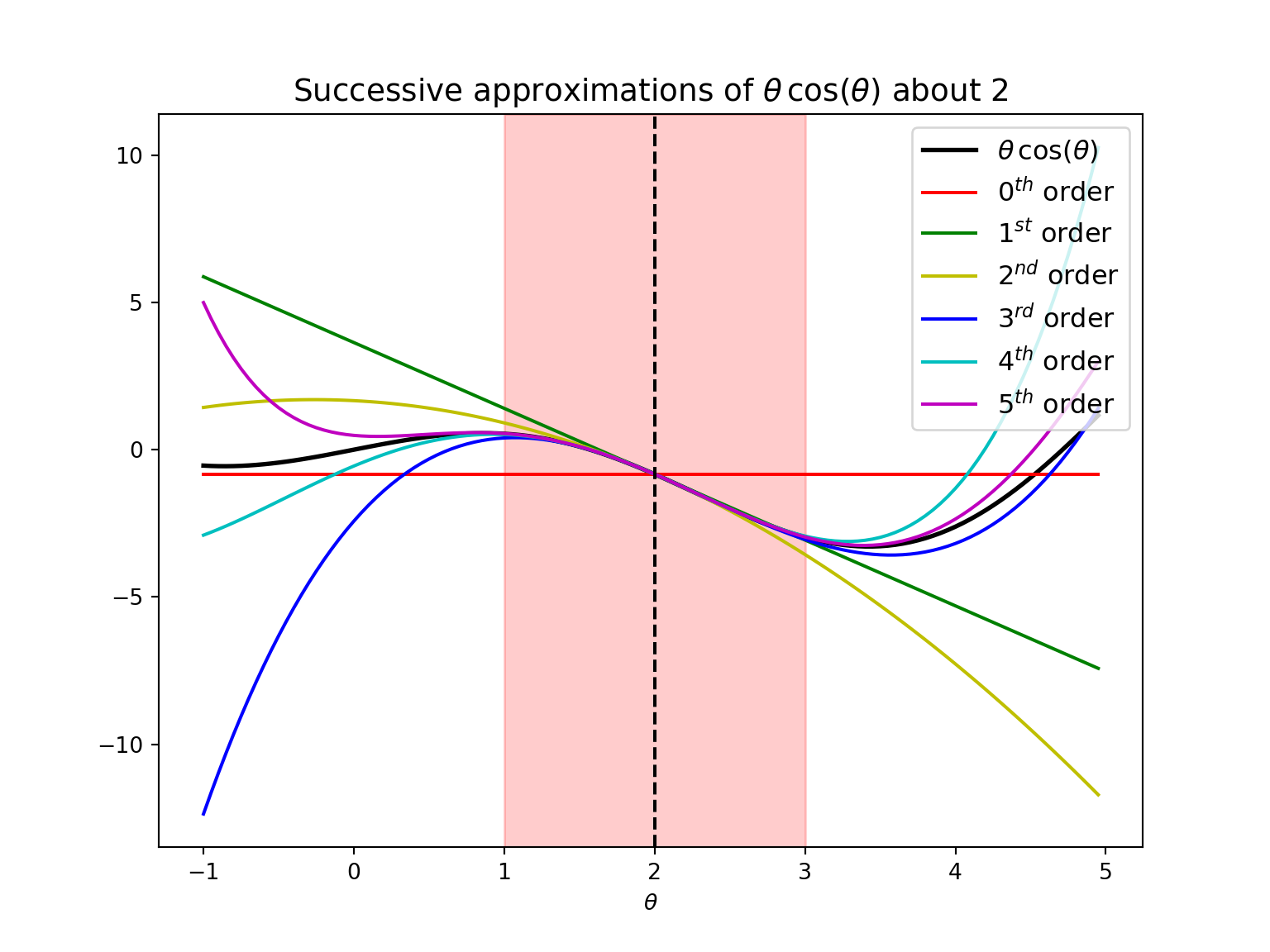
3.1.4 Taylor Expansion
Let \(f\) be a univariate smooth function. Taylor expansion of \(f\) about a point \(a\) is given by
The \(m^{th}\) order Taylor approximation of \(f\) is given by ignoring all the terms of order more than \(m\) in the Taylor expansion. That is,
\[f(\theta) \approx \sum_{i = 0}^m \frac{(\theta - a)^i}{i!} \frac{\mathrm{d}^i f(a)}{\mathrm{d} \theta^i}\]
is the \(m^{th}\) order Taylor approximation of \(f\) about \(a\).
Note that for \(m^{th}\) order approximations, we only need to compute the first \(m\) derivatives of the function.
Similarly, for a multivariate function \(f\), the Taylor expansion about a point \(\mathbf a\) is given by
\[f(\theta) = f(\mathbf a) + (\theta - \mathbf a)\boldsymbol{\cdot}\nabla f(\mathbf a) + \frac{1}{2} (\theta - \mathbf a) \boldsymbol{\cdot}\left(\nabla^2 f(\mathbf a) (\theta - \mathbf a)\right) + \cdots.\]
Then, by ignoring the terms of order more than \(m\), we get \(m^{th}\) order approximation of \(f\) about \(\mathbf a\).
3.2 General Framework of Local Descent Methods
In this section, we introduce a general framework of local descent methods.
- Given an \(n\)-dimensional multivariate function \(f : \Theta \to \mathbb R\) over a feasible set \(\Theta \subseteq \mathbb R^n\), the general approach of optimization is to incrementally take steps on \(\Theta\) based on a local model so that the function value \(f(\theta)\) is decreased. That is we want to solve the following optimization problem:
\[\begin{equation*} \min_{\theta \in \Theta} f(\theta). \end{equation*}\]
We can think of \(f\) being the cost function of a neural network where \(\theta\) represents an unknown vector of parameters taking values on a known set \(\Theta\), and the goal to find the value of \(\theta\) that minimizes the cost.
The optimization methods that follow the common approach of the following pseudocode are called descent direction methods.
Algorithm : General approach of descent direction methods
- \(\mathbf \theta \leftarrow \theta^{(1)}\) (Start with an initial design point \(\theta^{(1)} \in \Theta\))
- repeat
- Determine the descent direction \(\mathbf d\)
- Determine the step size of learning rate \(\alpha\)
- \(\theta \leftarrow \theta + \alpha \mathbf d\) (The next design point)
- until \(\theta\) satisfies a termination condition
- return \(\theta, f(\theta)\)
Following figure illustrates working of a descent direction method on a Rosenbrock function.
Different methods follow different approaches in finding the descent direction \(\mathbf d\) and step size or learning rate \(\alpha\). Similarly the termination condition in Step 6 can change from method to method.
For each \(k \geq 1\), denote the values of \(\theta\), \(\mathbf d\) and \(\alpha\) in the \(k\)-th iteration of the algorithm by \(\theta^{(k)}\), \(\mathbf d^{(k)}\) and \(\alpha^{(k)}\), respectively.
The descent direction \(\mathbf d^{(k+1)}\) of the next iteration is determined by the local information such as gradient and/or Hessian of the function \(f\) at \(\theta^{(k)}\). Some methods normalize the descent direction so that \(\|\mathbf d^{(k)}\| = 1\) for all \(k\).
The phrase step size is generally refers to the magnitude of the overall step, that is, step size in \(k\)-th iteration is equal to \(\alpha^{(k)}\|\mathbf d^{(k)} \|\). When \(\|\mathbf d^{(k)}\| = 1\), the learning rate \(\alpha\) is same as the step size.
In some algorithms, the step size is optimized so that it decreases the function \(f\) maximally. However, it may come at an extra computational cost.
In conclusion, different methods use different approaches to find \(\alpha\) and \(\mathbf d\).
3.3 Finding Step Size
In this section, we assume that the descent direction \(\mathbf d\) is given to us. Section 3.5 on first-order methods will deal with how to select \(\mathbf d\). Directional derivative plays a key role in finding the step size in each iteration.
3.3.1 Line Search
- Line search is used to find the optimal learning rate \(\alpha\) for a given descent direction \(\mathbf d\). That is, line search is a univariate optimization problem to find the solution of
Any univariate optimization method can be used for solving the above problem.
In many cases, the cost of the above optimization problem can be much higher. Instead, a reasonable value of \(\alpha\) can do the job.
It is indeed common to fix a sequence \(\alpha^{(1)}, \alpha^{(2)}, \dots\) in advance. In particular, a well-known method is to use decaying step factor: \[\alpha^{(k)} = \alpha^{(1)} \gamma^{k-1}, \, \, \text{for}\, \, k =1,2,\dots,\] for some \(\gamma \in [0, 1]\).
Decaying step factors are quite popular in machine learning when minimizing noisy functions.
Example: Consider the function
\[f(\theta) = \sin(\theta_1 \theta_2) + \exp(\theta_2 + \theta_3) - \theta_3,\] for \(\theta = (\theta_1, \theta_2, \theta_3) \in \mathbb{R}^3\). The goal is to find \(\alpha\) that solves (3.3) from \(\theta = (1,2,3)\) in the direction \(\mathbf d = [0, -1, -1]\).
Then the optimization problem (3.3) becomes: \[\begin{equation*} \min_{\alpha} \left[\sin(2 - \alpha) + \exp(5 - 2\alpha) + \alpha - 3\right]. \end{equation*}\]
That is the optimal \(\alpha\) is a solution of
\[f'(\alpha) = - \cos(2 - \alpha) - 2 \exp(5 - 2\alpha) + 1,\] which can be solved using any standard optimization method like Newton-Raphson method, as shown in the following python code.
import numpy as np
import matplotlib.pyplot as plt
from scipy import optimize

g = lambda alpha : - np.cos(2 - alpha) - 2*np.exp(5 - 2*alpha) + 1

x_values = np.arange(1, 6, 0.01)
y_values = [g(x_values[i]) for i in range(x_values.shape[0])]

sol = optimize.newton(g, 0)

plt.figure(figsize=(7,4))
## <Figure size 700x400 with 0 Axes>## [<matplotlib.lines.Line2D object at 0x7fb391b48b38>]## <matplotlib.lines.Line2D object at 0x7fb391b48da0>## Text(0.5, 0, '$\\alpha$')## Text(3.127045611348646, -44, '$\\alpha^*$')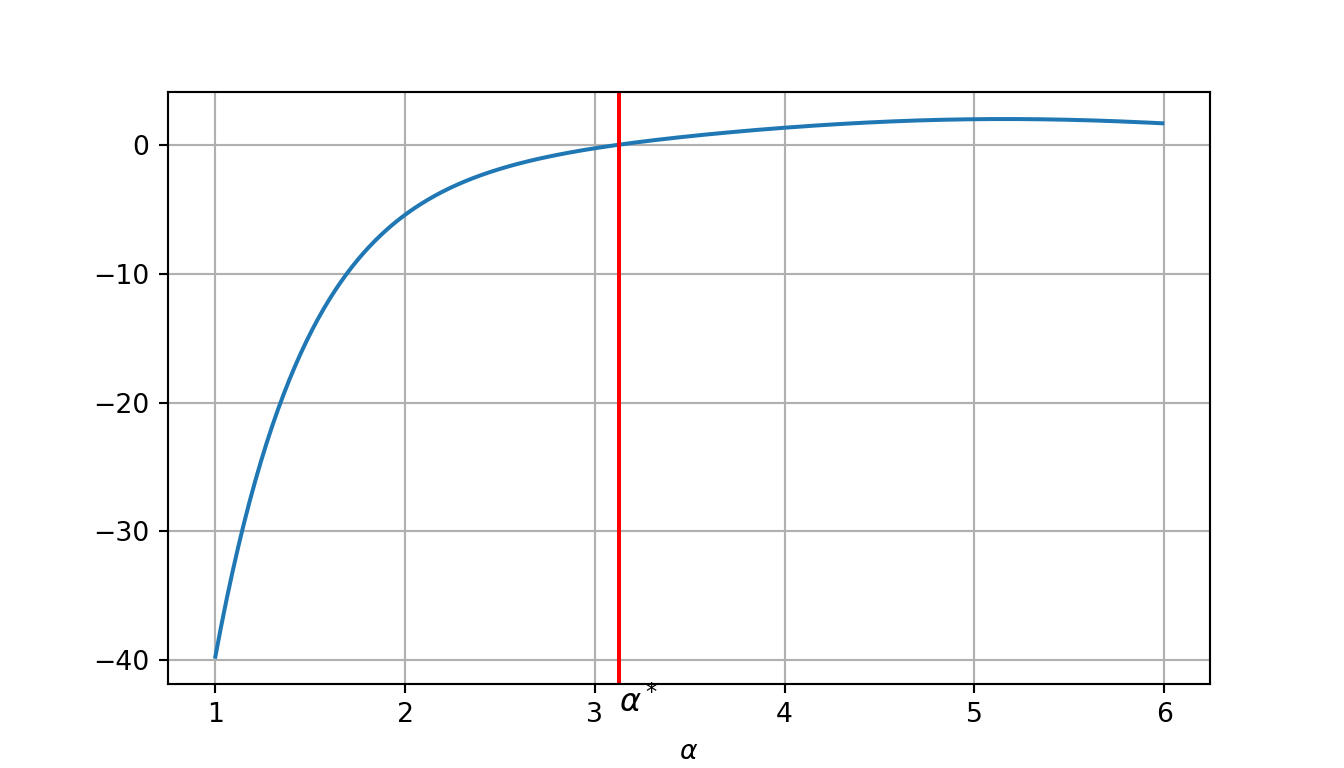
## Solution: 3.1270456113486463.3.2 Approximate Line Search
When solving the optimization problem in each iteration of the exact line search is expensive, it is economical to take more steps with approximate line search.
Sufficient decrease condition: Select the step size \(\alpha > 0\) and \(\beta \in [0,1]\) such that \[f(\theta^{(k+1)}) \leq f(\theta^{(k)}) + \beta \alpha \nabla_{\mathbf d^{(k)}} f(\theta^{(k)}),\] for a given descent direction \(\mathbf d^{(k)}\).
Sufficient decrease condition is also known as Armijo condition or the first Wolfe condition.
Typically, in practice, \(\beta\) is taken to be \(10^{-4}\).
Issue: The first Wolfe condition doesn’t guarantee convergence to a local minimum. This is because, very small steps can satisfy the condition and that can cause premature convergence.
Backtracking line search: To remedy the above issue, backtracking line search is used. In each iteration, a largest possible step size \(\alpha\) is taken. Then, decrease it sequentially until the sufficient decrease condition is satisfied. This guarantees convergence to a local minimum.
Example: Again consider Rosenbrock function,
The backtracking line search from \(\theta = [-0.5, 1.0]\) in the direction \(\mathbf d = [-1, -1.5]\). Initially \(\alpha = 1\), and at each iteration, it is decreased as \(\alpha \leftarrow \alpha/2\).
import numpy as np
import sympy

def backtracking_line_search(f, grad, t, d, a, p = 0.5, beta= 1e-4):
    f_lam = sympy.lambdify((t1, t2), f)
    z = f_lam(t[0], t[1])
    g = [s.subs([(t1, t[0]), (t2, t[1])]).evalf() for s in grad]
    theta_next = t + a*d

    while f_lam(theta_next[0], theta_next[1]) > z + a*beta*np.dot(g, d):
        a *= p
        theta_next = t + a*d
    return a


t1, t2 = sympy.symbols('t1, t2', real=True)
f = (1.0 - t1)**2 + 100*(t2 - t1**2)**2
theta = (t1, t2)
grad = [f.diff(t) for t in theta]


t = np.array([-0.5, 1.0])
d = np.array([-1, -1.5])
a_init = 1.0
sol = backtracking_line_search(f, grad, t, d, a_init)

print('Solution:', sol)
## Solution: 0.25Curvature condition: An alternative to Backtracking line search, the curvature condition requires that \[\nabla_{\mathbf d^{(k)}} f(\theta^{(k+1)}) \geq \sigma \nabla_{\mathbf d^{(k)}} f(\theta^{(k)}),\] where \(\sigma\) controls how shallow the next directional derivative should be. In practice it is common to take \(\beta < \sigma < 1\), with \(\sigma = 0.1\) when it is used for the conjugate gradient method and \(\sigma = 0.9\) when it is used for Newton’s method.
Strong Wolfe condition: It is an alternative to and stronger than the curvature condition. Strong Wolfe condition: \[|\nabla_{\mathbf d^{(k)}} f(\theta^{(k+1)})| \leq -\sigma \nabla_{\mathbf d^{(k)}} f(\theta^{(k)}).\]
Wolfe conditions: The sufficient decrease condition and the curvature condition together are called the Wolfe conditions, which guarantee convergence to a local minimum.
strong Wolfe conditions: The sufficient decrease condition and the strong Wolfe condition together are called the strong Wolfe conditions, which again guarantee convergence to a local minimum.
Exercise: Conduct approximate line search on \(f(\theta) = \theta_1^2 + \theta_1 \theta_2 + \theta_2^2\) from \(\theta = [1,2]\) in the direction \(\mathbf d = [-1,-1]\) such that the Wolfe conditions satisfy.
Take the maximum step size to be \(10\) (i.e., start with \(\alpha^{(1)} = 10\)), reduction factor \(\gamma = 0.5\) (i.e., in \(k^{th}\) iteration \(\alpha^{(k)} = \alpha^{(1)} \gamma^{k-1}\)), the first Wolfe condition parameter \(\beta = 10^{-4}\), and the second Wolfe condition parameter \(\sigma = 0.9\).
Hint: The Wolfe conditions will be satisfied on the \(3^{rd}\) iteration, and the final \(\alpha = 2.5\) and the final \(\theta = [-1.5, -0.5]\).
Exercise: Recall that for any point \(\theta\) and direction \(\mathbf d\), the Wolfe condition is
\[f(\theta + \alpha \mathbf d) \leq f(\theta) + \beta \alpha \nabla_{\mathbf d} f(\theta).\]
For \(f(\theta) = 4 + 2\theta_1^2 + \theta_2^2\), find the maximum stepsize \(\alpha\) that satisfies this condition when \(\theta = [-1,-1]\), \(\mathbf d = [1,0]\), and \(\beta = 10^{-5}\).
3.4 Termination Conditions
Here, we discuss four commonly used termination conditions.
Maximum number of iterations: Under this condition, the algorithm is terminated either when the number of iterations exceeds a pre-selected number \(k_\max\), or the total running time of the algorithm exceeds a pre-selected time \(t_\max\). This is useful when there is a strict running time constraint, because for all the other termination conditions mentioned baove, it is hard to say hong the algorithm takes to terminate.
The plot in Section~3.5.6 compares the performance of different gradient methods with the same \(k_\max\). Evidently, it will be clear that the same choice of \(k_\max\) does not work for all the methods.Absolute Improvement: Algorithm is terminated if the change in the function value is smaller than a pre-selected threshold \(\epsilon_a\) over subsequent steps. That is, the termination condition is, \[ |f(\theta^{(k)}) - f(\theta^{(k+1)})| < \epsilon_a.\]
Gradient Magnitude: Algorithm is terminated if the magnitude \(\| \nabla f(\theta^{(k+1)}) \|\) of the derivative is smaller than a pre-selected threshold \(\epsilon_g\), that is, \[\| \nabla f(\theta^{(k+1)}) \| < \epsilon_g.\]
Relative Improvement: Algorithm is terminated if the relative change \(\frac{|f(\theta^{(k)}) - f(\theta^{(k+1)})|}{|f(\theta^{(k)})|}\) is smaller than a pre-selected threshold \(\epsilon_r\) over subsequent steps. That is, the termination condition is
\[ |f(\theta^{(k)}) - f(\theta^{(k+1)})| < \epsilon_r |f(\theta^{(k)})|.\] Relative improvement condition is particularly useful when the region around the (local) minimum is shallow.
Example: For instance, in the following figure, we see surface plots for
\[\begin{eqnarray*} f_1(\theta) = \theta_1^2 + \theta_2^2,\quad \color{blue}{\text{Blue Surface}} \end{eqnarray*}\]
and \[\begin{eqnarray*} f_2(\theta) = 0.2\theta_1^2 + 0.2\theta_2^2. \quad \color{red}{\text{Red Surface}} \end{eqnarray*}\]
Both of these functions have global minimum at \((0,0)\). However, \(f_2\) is shallower around \((0,0)\) than \(f_1\).
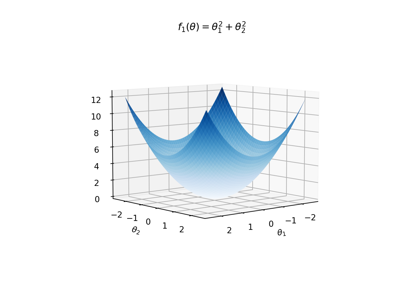
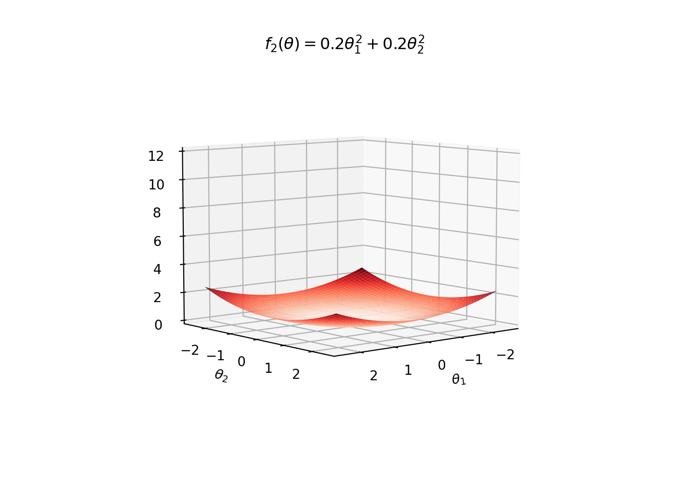
Suppose that a descent direction algorithm takes a step of size \(0.2\) in each iteraction. We see that the relative improvement condition works well for both the functions.
Absolute Improvement: First assume that the algorithm uses the absolute improvement condition with \(\epsilon_a = 0.1\). Then for \(f_1\), \(\theta^{(k)}\) should be within the blue cicle (in the figure below) before the termination, while for \(f_2\), the algorithm can terminate when \(\theta^{(k)}\) takes a value within the red circle.
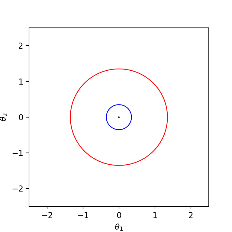
Gradient Magnitude: Assume that the gardient magnitude condition with \(\epsilon_g = 0.1\) in the algorithm. Then the algorithm terminates for \(f_1\) when \(\theta^{(k+1)}\) is within the blue circle shown in the following figure, while for \(f_2\) it terminates when \(\theta^{(k+1)}\) is within the red circle.
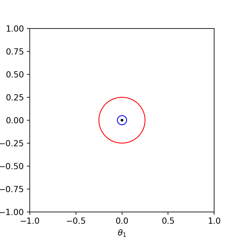
Relative Improvement: Finally assume that the algorithm uses the relative improvement condition with \(\epsilon_r = 0.1\) for the termination. Then for both the functions, the algorithm terminates only when \(\theta^{(k)}\) is within the circle centered at the origion with radius \(\approx 0.097\). This is because the relative improvement is the same for both the functions, i.e.,
\[ \frac{|f_1(\theta^{(k)}) - f_1(\theta^{(k+1)})|}{|f_1(\theta^{(k)})|} = \frac{|f_2(\theta^{(k)}) - f_2(\theta^{(k+1)})|}{|f_2(\theta^{(k)})|}, \]
for any \(\theta^{(k)}\) and \(\theta^{(k+1)}\).
3.5 First-Order Methods
Finally, we focus on the most important aspect of the local descent methods: finding the descent direction \(\mathbf d\). As mentioned earlier, first-order methods use the gradient of the function for selecting appropriate descent direction \(\mathbf d\) in each iteration.
3.5.1 Gradient Descent
An obvious choice for the descent direction is in the direction of steepest descent.
Steepest descent direction guarantees an improvement, provided that the function is smooth, the step size is sufficiently small, and we are not at a minimum point (i.e., non-zero gradient).
Again let \(\theta^{(k)}\) be the design point in the \(k\)-th iteration. Define,
\[g^{(k)} = \nabla f(\theta^{(k)}).\]
The steepest direction in the \(k\)-th iteration is the direction opposite the gradient \(g^{(k)}\) (hence the name gradient descent).
The descent direction \(\mathbf d^{(k)}\) is typically the normalized steepest descent, that is, \[\mathbf d^{(k)} = - \frac{g^{(k)}}{\|g^{(k)}\|},\] where the negative sign implies that the descent direction is opposite the gradient.
Observation: If the step size \(\alpha^{(k)}\) is selected using exact line search: \[\alpha^{(k)} = \underset{\alpha}{\arg \min} f(\theta^{(k)} + \alpha \mathbf d^{(k)}),\] then the gradient descent can result in zig-zagging. To see this, observe that \[f'(\theta^{(k)} + \alpha^{(k)} \mathbf d^{(k)}) = \frac{\partial f(\theta^{(k)} + \alpha \mathbf d^{(k)})}{\partial \alpha} = 0.\] Consequently, the directional derivative \(\nabla_{\mathbf d^{(k)}} f(\theta^{(k)} + \alpha^{(k)}\mathbf d^{(k)}) = 0\), because \[\begin{align*} 0 &= f'(\theta^{(k)} + \alpha^{(k)} \mathbf d^{(k)})\\ &= \lim_{h \to 0} \frac{f(\theta^{(k)} + (\alpha^{(k)} + h) \mathbf d^{(k)}) - f(\theta^{(k)} + \alpha^{(k)} \mathbf d^{(k)})}{h}\\ &= \lim_{h \to 0} \frac{\nabla f(\theta^{(k)} + \alpha^{(k)}\mathbf d^{(k)}) \boldsymbol{\cdot}(h \mathbf d^{(k)}) + O(h^2)}{h}\\ &= \nabla f(\theta^{(k)} + \alpha^{(k)}\mathbf d^{(k)}) \boldsymbol{\cdot}\mathbf d^{(k)}\\ &= \nabla_{\mathbf d^{(k)}} f(\theta^{(k)} + \alpha^{(k)}\mathbf d^{(k)}). \end{align*}\] Since \[ \mathbf d^{(k + 1)} = - \frac{\nabla f(\theta^{(k)} + \alpha^{(k)}\mathbf d^{(k)})}{\|\nabla f(\theta^{(k)} + \alpha^{(k)}\mathbf d^{(k)}) \|},\] we have \[\mathbf d^{(k+1)}\boldsymbol{\cdot}\mathbf d^{(k)} = 0.\] That is, the descent direction in each iteration is perpendicular to the descent direction of the previous iteration. Therefore, we obtain jagged search paths.
Example: Consider Booth’s function, a 2-dimensional quadratic function: \[f(\theta) = (\theta_1 + 2\theta_2 - 7)^2 + (2\theta_1 + \theta_2 - 5)^2.\] This has a global minimum at \((1,3)\). The following code implements gradient-descent method with exact line search. We start with \(\theta^{(1)} = [-9, 8]\).
def f(t):
    return (t[0] + 2*t[1] - 7)**2 + (2*t[0] + t[1] -5)**2

def grad(t):
    return np.array([10*t[0] + 8*t[1] - 34, 8*t[0] + 10*t[1] - 38])

def line_search_exact(t, d):
    nume = (t[0] + 2*t[1] - 7)*(d[0] + 2*d[1]) + (2*t[0] + t[1] - 5)*(2*d[0] + d[1])
    deno = (d[0] + 2*d[1])**2 + (2*d[0] + d[1])**2
    return -nume/deno

def GradientDescent_exact(f, grad, t, niter):
    g = grad(t)
    norm = np.linalg.norm(g)
    d = -g/norm
    t_seq = [t]
    d_seq = [d]

    for _ in range(niter):
        alpha = line_search_exact(t, d)

        # Theta update
        t = t + alpha*d
        t_seq.append(t)

        g = grad(t)
        norm = np.linalg.norm(g)
        d = -g/norm
        d_seq.append(d)

    print('Final point of GD:', t)
    t_seq = np.array(t_seq)
    d_seq = np.array(d_seq)
    return t_seq, d_seq

t_init = np.array([-9.0, 8.0])

t1_range = np.arange(-10.0, 10.0, 0.05)
t2_range = np.arange(-10.0, 10.0, 0.05)
A = np.meshgrid(t1_range, t2_range)
Z = f(A)

fig, ax = plt.subplots()
ax.contour(t1_range, t2_range, Z, levels=np.exp(np.arange(-10, 6, 0.5)), cmap='Blues')ax.plot(t_seq_gd[:, 0], t_seq_gd[:, 1], '-r', label=r'Exact $\alpha$')
plt.xlabel(r'$\theta_1$')
plt.ylabel(r'$\theta_2$')
plt.legend()
plt.show()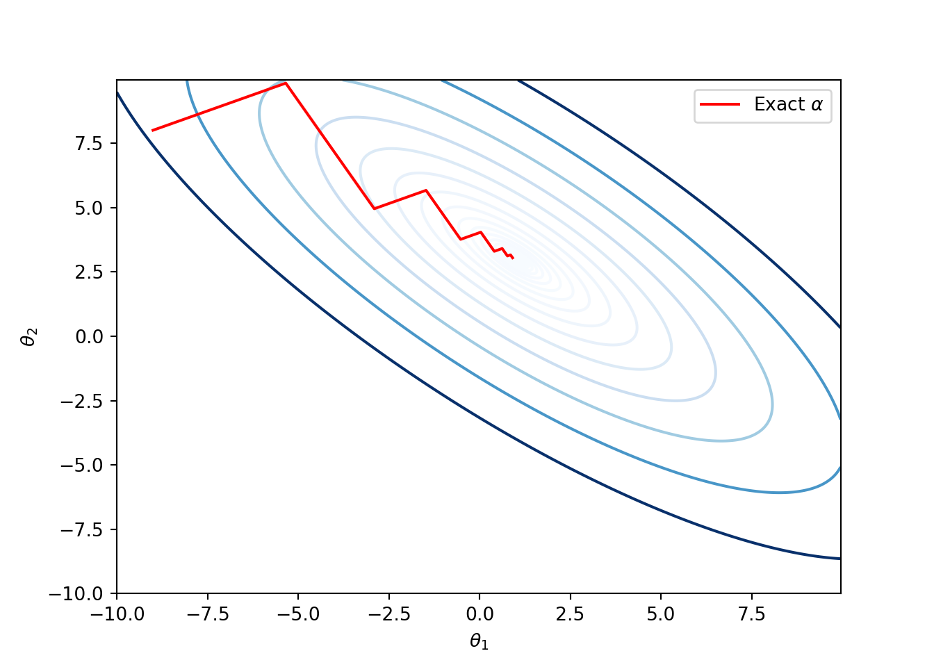
Run the following lines to print the sequence of directions \(\mathbf d^{(1)}, \mathbf d^{(2)}, \dots\), the sequence of parameters \(\theta^{(1)}, \theta^{(2)}, \dots\), and the gradient vectors \(g^{(1)}, g^{(2)}, \dots\).
for i in range(len(d_seq_gd)):
  print('iteration:', i+1)
  print('\t d = ', d_seq_gd[i])
  print('\t t = ', t_seq_gd[i])
  print('\t Gradient =', grad(t_seq_gd[i]))
Example: Since, the gradient descent method follows the steepest descent direction, ideally speaking it should behave like water flowing from \(\theta^{(1)}\) and eventually reaching the local minimum. This happens when the step size is very small as illustrated in the following figure. They key drawback of small step size is that the number computations can drastically increase compared to the earlier exact line search version. For instance, in the following code we used \(10\) iterations for the exact line search and \(10,000\) for the small step size of \(0.001\).
def GradientDescent_fixed(f, grad, t, alpha,  niter):
    g = grad(t)
    norm = np.linalg.norm(g)
    d = -g/norm
    t_seq = [t]
    d_seq = [d]

    for _ in range(niter):
        # Theta update
        t = t + alpha*d
        t_seq.append(t)

        g = grad(t)
        norm = np.linalg.norm(g)
        d = -g/norm
        d_seq.append(d)

    print('Final point of GD:', t)
    t_seq = np.array(t_seq)
    d_seq = np.array(d_seq)
    return t_seq, d_seq

alpha = 0.001
t_init = np.array([-9.0, 8.0])

t1_range = np.arange(-10.0, 10.0, 0.05)
t2_range = np.arange(-10.0, 10.0, 0.05)
A = np.meshgrid(t1_range, t2_range)
Z = f(A)

fig, ax = plt.subplots()
ax.contour(t1_range, t2_range, Z, levels=np.exp(np.arange(-10, 6, 0.5)), cmap='Blues')
ax.plot(t_seq_gd[:, 0], t_seq_gd[:, 1], '-r', label=r'Exact $\alpha$')
t_seq_gd_fixed, d_seq_gd_fixed = GradientDescent_fixed(f, grad, t_init, alpha, niter=10000)ax.plot(t_seq_gd_fixed[:, 0], t_seq_gd_fixed[:, 1], '-b', label=r'Fixed $\alpha = 0.001$')
plt.xlabel(r'$\theta_1$')
plt.ylabel(r'$\theta_2$')
plt.legend()
plt.show()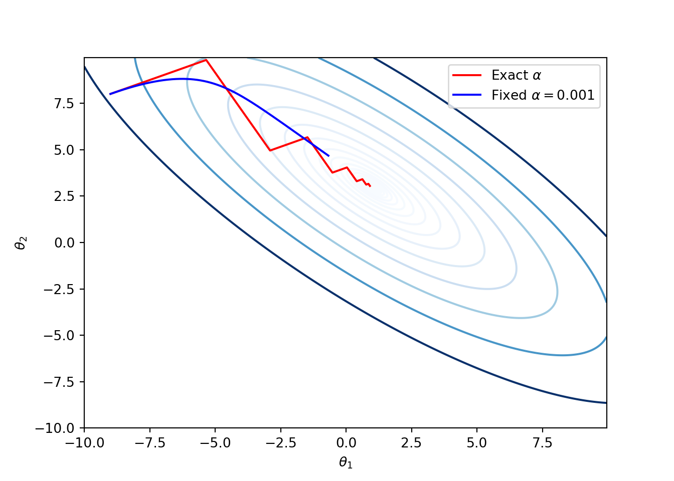
Exercise: For the above Booth’s function, prove that the global minimum is achieved at \(\theta^* = (1,3)\) by solving \(\nabla f(\theta) = 0\), and find the value of \(f(\theta^*)\).
3.5.2 Cojugate Gradient
Performance of the gradient descent method can be poor in narrow valleys. The conjugate descent method addresses this issue.
The Conjugate gradient method works well for optimizing quadratic functions: \[f(\theta) = \frac{1}{2}\theta \boldsymbol{\cdot}\left(\mathbf A \theta\right) + \mathbf b \boldsymbol{\cdot}\theta + c,\] where \(\mathbf A\) is a symmetric positive definite matrix. Then the optimization problem \[\min_{\theta} f(\theta)\] has a unique solution.
The descent directions of the algorithm are chosen so that they are mutually conjugate with respect to \(\mathbf A\), that is, \[\mathbf d^{(i)} \boldsymbol{\cdot}\left( \mathbf A \mathbf d^{(j)}\right) = 0,\quad \text{for all}\, \, i \neq j.\]
The algorithm uses line search in each iteration to find the step factor \(\alpha\). It is an easy problem for quadratic functions. Because to solve \(\min_{\alpha} f(\theta + \alpha \mathbf d)\), we can easily solve
\[\frac{\partial f(\theta + \alpha \mathbf d)}{\partial \alpha} = 0.\] Observe that
\[\begin{align*} \frac{\partial f(\theta + \alpha \mathbf d)}{\partial \alpha} &= \mathbf d \boldsymbol{\cdot}\mathbf A(\theta + \alpha \mathbf d) + \mathbf d \boldsymbol{\cdot}\mathbf b\\ &= \mathbf d \boldsymbol{\cdot}(\mathbf A\theta + \mathbf b) + \alpha \mathbf d \boldsymbol{\cdot}\mathbf A \mathbf d. \end{align*}\] Equating this to zero results in \[\alpha = - \frac{\mathbf d \boldsymbol{\cdot}(\mathbf A\theta + \mathbf b)}{\mathbf d \boldsymbol{\cdot}\mathbf A \mathbf d}.\]The algorithm starts in the steepest descent direction: \[\mathbf d^{(1)} = -g^{(1)} = - \nabla f(\theta^{(1)}).\] So, \[\theta^{(2)} = \theta^{(1)} + \alpha^{(1)} \mathbf d^{(1)}.\]
In the subsequent iterations \[\mathbf d^{(k+1)} = - g^{(k+1)} + \beta^{(k)} \mathbf d^{(k)} = - \nabla f(\theta^{(k+1)}) + \beta^{(k)} \mathbf d^{(k)},\] where the scalar parameter \(\beta^{(k)}\) is selected so that \(\mathbf d^{(k)}\) and \(\mathbf d^{(k+1)}\) are mutually conjugate with respect to \(\mathbf A\), as shown below: \[\begin{align*} \mathbf d^{(k+1)} \boldsymbol{\cdot}\mathbf A \mathbf d^{(k)} &= 0\\ \Rightarrow ( - g^{(k+1)} + \beta^{(k)} \mathbf d^{(k)}) \boldsymbol{\cdot}\left(\mathbf A \mathbf d^{(k)}\right) &= 0\\ \Rightarrow - g^{(k+1)} \boldsymbol{\cdot}\left(\mathbf A \mathbf d^{(k)}\right) + \beta^{(k)} (\mathbf d^{(k)}) \boldsymbol{\cdot}\left(\mathbf A \mathbf d^{(k)} \right)&= 0\\ \Rightarrow \beta^{(k)} = \frac{g^{(k+1)} \boldsymbol{\cdot}\left(\mathbf A \mathbf d^{(k)}\right)}{(\mathbf d^{(k)} \boldsymbol{\cdot}\left(\mathbf A \mathbf d^{(k)}\right)}. \end{align*}\]
Example: Again consider the Booth’s function from the previous example:
\[f(\theta) = (\theta_1 + 2\theta_2 - 7)^2 + (2\theta_1 + \theta_2 - 5)^2.\]
The following code implements the conjugate gradient method.
def ConjGradientDescent_exact(f, grad, t, A, b, niter):
    g = grad(t)
    d = -g
    t_seq = [t]
    d_seq = [d]

    for _ in range(niter):
        alpha = line_search_exact(t, d)

        # Theta update
        t = t + alpha*d

        g = grad(t)
        Ad = A@d
        beta = np.dot(g, Ad)/(np.dot(d, Ad))
        d = -g + beta*d
        if np.linalg.norm(d) < 10e-16:
            t_seq = np.array(t_seq)
            d_seq = np.array(d_seq)
            return t_seq, d_seq
        t_seq.append(t)
        d_seq.append(d)

    print('Final point of GD:', t)
    t_seq = np.array(t_seq)
    d_seq = np.array(d_seq)
    return t_seq, d_seq

A = np.array([[10, 8], [8, 10]])
b = -np.array([34, 38])

t1_range = np.arange(-10.0, 10.0, 0.05)
t2_range = np.arange(-10.0, 10.0, 0.05)
XY = np.meshgrid(t1_range, t2_range)
Z = f(XY)
plt.contour(t1_range, t2_range, Z, levels=np.exp(np.arange(-3, 7, 0.5)), cmap='Blues')t_seq_cgd, _ = ConjGradientDescent_exact(f, grad, t_init, A, b, niter=10)
plt.plot(t_seq_cgd[:, 0], t_seq_cgd[:, 1], '-r', label='CGD')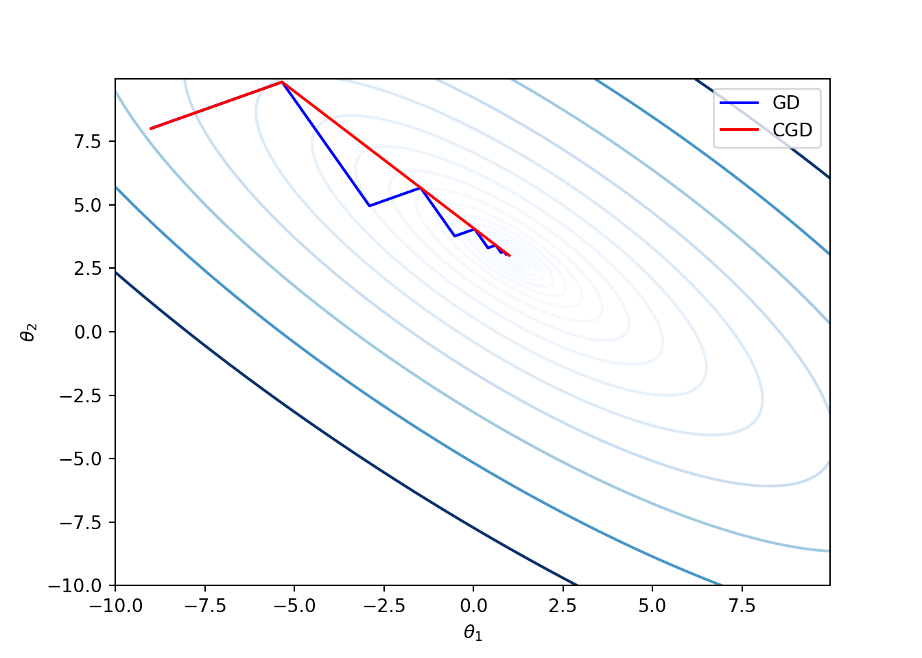
The above figure illustrates that the conjugate gradient method can have faster convergence compared to the gradient descent method.
-
The conjugate method can also be applied to non-quadratic functions as well because smooth continuous functions behave like quadratic functions close to the minimum. However, unfortunately, it is hard to find \(\mathbf A\) that best approximates \(f\) locally. Observe that \(\mathbf A\) is needed for computing \(\beta\) values. The following choices for \(\beta^{(k)}\) seems to work well in practice.
Fletcher-Reeves: \[\beta^{(k)} = \frac{g^{(k)}\boldsymbol{\cdot}g^{(k)}}{g^{(k-1)} \boldsymbol{\cdot}g^{(k-1)}}.\]
Polak-Ribiere: \[\beta^{(k)} = \frac{g^{(k)} \boldsymbol{\cdot}(g^{(k)} - g^{(k-1)})}{g^{(k-1)} \boldsymbol{\cdot}g^{(k-1)}}.\]
Exercise: Modify and run the python code for conjugate gradient with the above two choices of \(\beta\) update.
3.5.3 Challenges Posed by the Above Gradient Descent Methods
Gradient descent methods offer a few important challenges that meed to be addressed to make them useful in the neural network set-up.
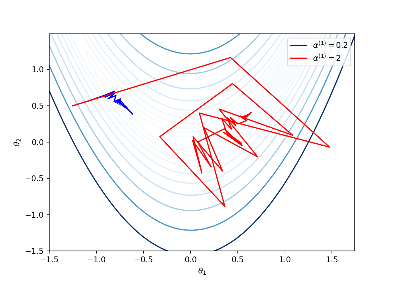
- Selection of the learning rate can be difficult. Small values of learning rate can result in slow convergence and large values can result in the loss function to fluctuate around the minimum, or even diverge. The following figure shows applications of the gradient descent method for Rosenbrock function given in (3.4) with two choices of \(\alpha^{(1)}\), where the learning rates are updated as \(\alpha^{(k + 1)} = (0.9)^{k-1} \alpha^{(1)}\).
Some gradient descent methods try to adjust the learning rate during training by reducing the rate according to a pre-defined schedule or when the change in cost function between epochs falls below a threshold. These schedules and thresholds are unable to adapt to the characteristics of the dataset as they are defined in advance.
Applying the same learning rate to all parameter updates might not be a good idea as larger updates on rarely occurring features may result in faster convergences.
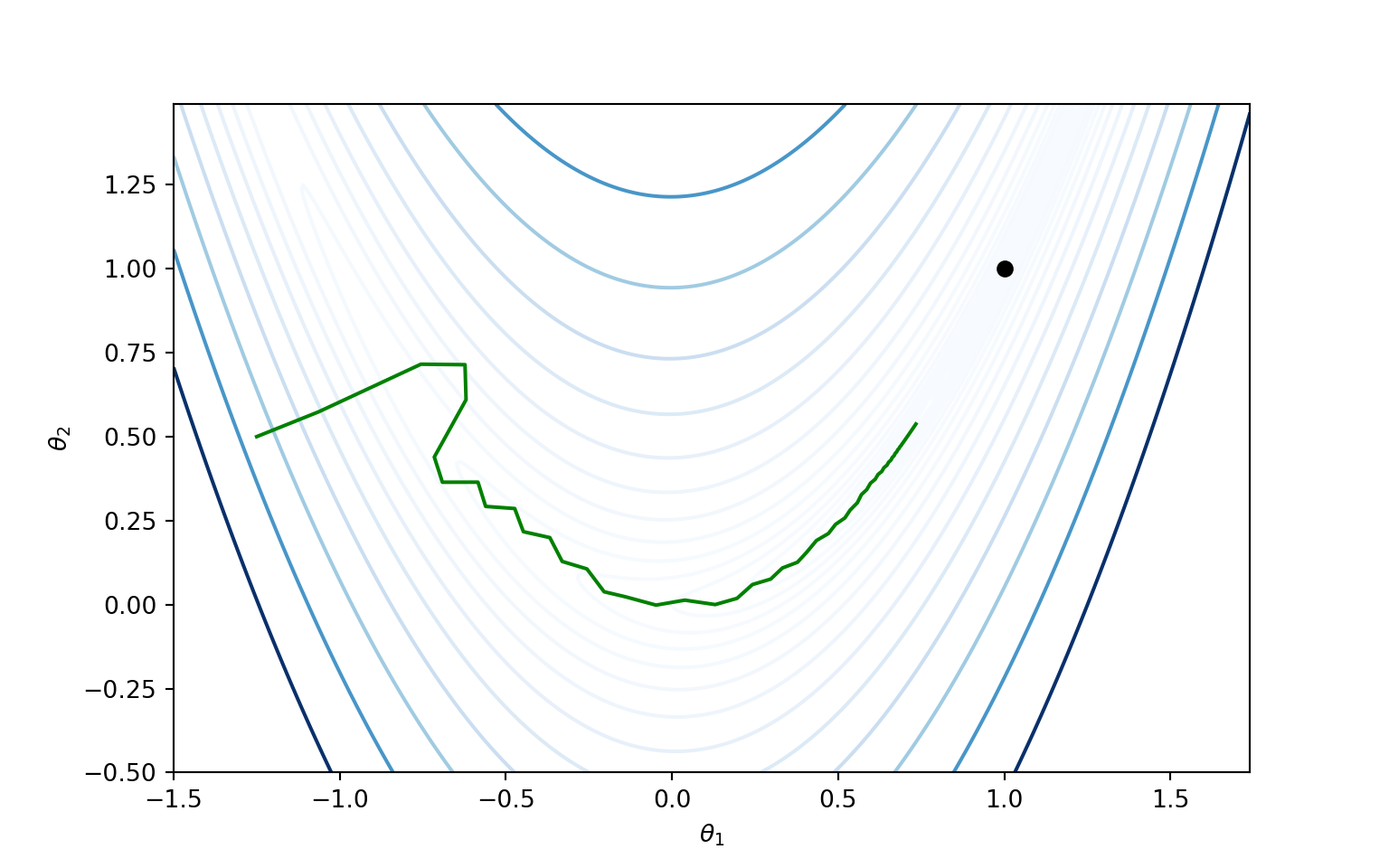
Gradient descent methods take time to traverse plateaus surrounding saddle points as the gradient in this region is close to zero in all directions.
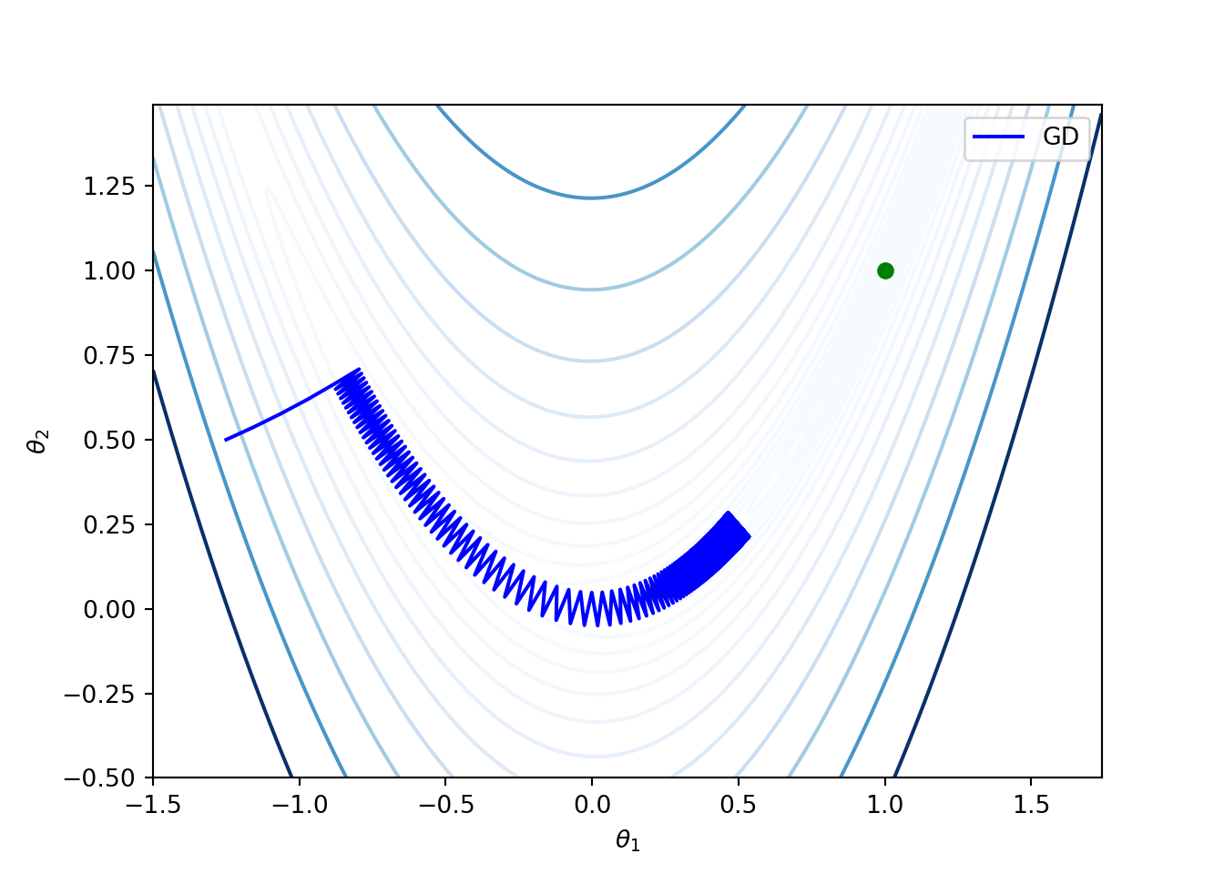
For instance, once again consider the Rosenbrock function given in (3.4). Note that for this function, the global minimum is achieved at \((1,1)\). The following figure shows that the gradient descent method is slow along the valley. This is because the gradient over a nearly flat region has small magnitude, and thus the gradient descent method can require many iterations to converge to a local minimum (same as the global minimum for the Rosenbrock function). The this experiment, the initial point \(\theta^{(1)} = (-1.25, 0.5)\), and the learning rate is fixed at \(\alpha = 0.1\).
From now onwards, we focus on a sequence of modified gradient descent methods for addressing the above issues.
3.5.4 Momentum
As mentioned above, the gradient methods take a long time to traverse over almost flat surfaces. Incorporating momentum accelerates the algorithm in the relevant directional and dampens oscillations.
The momentum updates at the \(k\)-the iteration are
\[\begin{align*} \mathbf v^{(k+1)} &= \beta \mathbf v^{(k)} - \alpha g^{(k)}\\ \theta^{(k+1)} &= \theta^{(k)} + \mathbf v^{(k+1)}, \end{align*}\] for a scalar parameter \(\beta\). When \(\beta = 0\), we have the standard gradient descent method.Interpretation: Think of a ball rolling down a nearly flat surface. Due to the gravity, the ball accumulates momentum as it rolls down, becoming faster and faster with time.
3.5.5 Nesterov Momentum
One problem with the momentum is that the steps do not slow down enough near the local minimum at the bottom of the valley. Hence, it has a tendency to overshoot the valley floor.
For the ball rolling scenario, we would want to the ball to be smart enough know where it is going to be in the next step so that it can slow down before the hill slopes up again.
Nesterov momentum captures this notion by using the gradient at the projected future position. The update is given by, \[\begin{align*} \mathbf v^{(k+1)} &= \beta \mathbf v^{(k)} - \alpha \nabla f(\theta^{(k)} + \beta \mathbf v^{(k)})\\ \theta^{(k+1)} &= \theta^{(k)} + \mathbf v^{(k+1)}, \end{align*}\]
Example: We once again consider the Rosenbrock function given by (3.4). The following code compares the basic gradient descent, momentum, and Nesterov momentum methods. We start with \(\theta^{(1)} = (-1.25, 0.5)\) and \(\alpha^{(1)} = 0.2\). The learning rate decreases as \(\alpha^{(k)} = \alpha^{(1)} \gamma^{k-1}\) where \(\gamma = 0.9\). For momentum and Nesterov momentum methods, we have taken \(\beta = 0.8\).
f = lambda t: (1 - t[0])**2 + 100*(t[1] - t[0]**2)**2

def grad(t):
    dx = -2*(1 - t[0]) - 4*100*t[0]*(t[1] - (t[0]**2))
    dy = 2*100*(t[1] - (t[0]**2))
    return np.array([dx, dy])

def GradientDescent(f, grad, t, alpha, gamma, niter=100000):
    g = grad(t)
    norm = np.linalg.norm(g)
    d = -g/norm
    t_seq = [t]
    d_seq = [d]

    for _ in range(niter):
        alpha *= gamma
        t = t + alpha*d
        t_seq.append(t)

        g = grad(t)
        norm = np.linalg.norm(g)
        d = -g/norm
        d_seq.append(d)

    t_seq = np.array(t_seq)
    d_seq = np.array(d_seq)
    return t_seq, d_seq

def MomentumGradientDescent(f, grad, t, alpha, gamma, beta, niter=100000):
    v = np.zeros(t.shape[0])
    t_seq = [t]
    v_seq = [v]

    for _ in range(niter):
        g = grad(t)
        norm = np.linalg.norm(g)
        v = beta*v - alpha*g/norm
        v_seq.append(v)

        alpha *= gamma
        t = t + v
        t_seq.append(t)

    t_seq = np.array(t_seq)
    v_seq = np.array(v_seq)
    return t_seq, v_seq

def NesterovMomentumGradientDescent(f, grad, t, alpha, gamma, beta, niter=100000):
    g = grad(t)
    norm = np.linalg.norm(g)
    v = np.zeros(t.shape[0])
    t_seq = [t]
    v_seq = [v]


    for _ in range(niter):
        g = grad(t + beta*v)
        norm = np.linalg.norm(g)
        v = beta*v - alpha*g/norm
        v_seq.append(v)

        alpha *= gamma
        t = t + v
        t_seq.append(t)

    t_seq = np.array(t_seq)
    v_seq = np.array(v_seq)
    return t_seq, v_seq

# Initialization
alpha_init = 0.2
gamma = 0.9
beta = 0.8
t_init = np.array([-1.25, 0.5])
niter = 100000

t1_range = np.arange(-1.5, 1.75, 0.01)
t2_range = np.arange(-0.5, 1.5, 0.01)

A = np.meshgrid(t1_range, t2_range)
Z = f(A)
plt.contour(t1_range, t2_range, Z, levels=np.exp(np.arange(-10, 6, 0.5)), cmap='Blues')
t_seq_gd, d_seq_gd = GradientDescent(f, grad, t_init, alpha_init, gamma, niter)
plt.plot(t_seq_gd[:, 0], t_seq_gd[:, 1], '-b', label='GD')t_seq_mgd, d_seq_mgd = MomentumGradientDescent(f, grad, t_init, alpha_init, gamma, beta, niter)
plt.plot(t_seq_mgd[:, 0], t_seq_mgd[:, 1], '-r', label='MGD')t_seq_nmgd, d_seq_nmgd = NesterovMomentumGradientDescent(f, grad, t_init, alpha_init, gamma, beta, niter)
plt.plot(t_seq_nmgd[:, 0], t_seq_nmgd[:, 1], '-g', label='NMGD')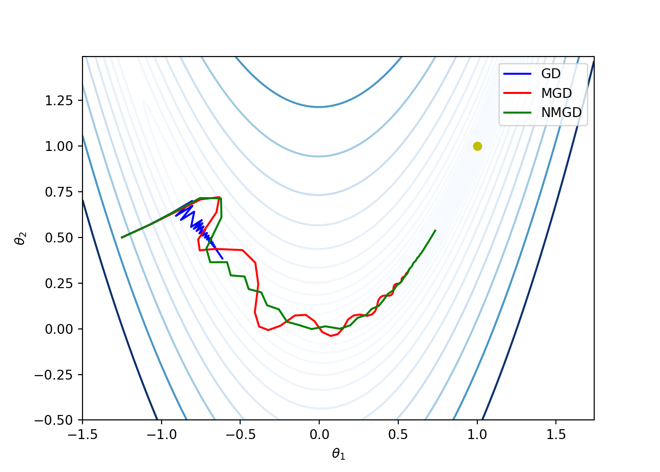
3.5.6 Adagrad
Observe that both momentum and Nesterov momentum methods update all components of \(\theta\) with the same learning rate.
The adaptive subgradient, or simply adgrad, adapts a learning rate for each component of \(\theta\) so that the components with frequent updates have low learning rates and the components with infrequent updates have high learning rate. As a consequence, it increases the influence of components of \(\theta\) with infrequent updates.
The update of each component in \(\theta\) is as follows. \[\begin{align*} \theta_i^{(k+1)} = \theta_i^{(k)} - \frac{\alpha}{\epsilon + \sqrt{s_i^{(k)}}} g_i^{(k)}, \end{align*}\] where \[ s_i^{(k)} = \sum_{j =1}^k \left(g_i^{(j)} \right)^2, \] \(g_i^{(k)}\) is the \(i\)-th component of \(g^{(k)}\), \(\epsilon\) is a small value of order \(1\times 10^{-8}\) to avoid division by zero, and \(\alpha\) is the learning rate parameter.
The adagrad method is less sensitive to the parameter \(\alpha\), which is typically set to be \(0.01\).
Drawback: The key drawback of the adagrad is that each component \(s_i\) is strictly non-deceasing. As a consequence the accumulated sum keeps increasing and hence the effective learning rate decreases during training, often making the effective learning rate infinitesimally small before convergence.
The first-order methods discussed below overcome this drawback.
Example: The following python function implements the adagrad method for the earlier example on Rosenbrock function. The corresponding plot compares the other methods with the adagrad method. The parameters chosen are \(\alpha = 0.01\) and \(\epsilon = 10^{-8}\).
def Adagrad(f, grad, t, alpha = 0.01, epsilon=10e-8, niter=100000):

    t_seq = [t]
    s = np.zeros(t.shape[0])

    #while norm > 10**(-8):
    for _ in range(niter):
        g = grad(t)
        norm = np.linalg.norm(g)
        g = g/norm

        s += np.multiply(g, g) # element-wise multiplication
        d = -np.divide(g, epsilon + np.sqrt(s)) # element-wise division
        t = t + alpha*d
        t_seq.append(t)

    t_seq = np.array(t_seq)
    return t_seq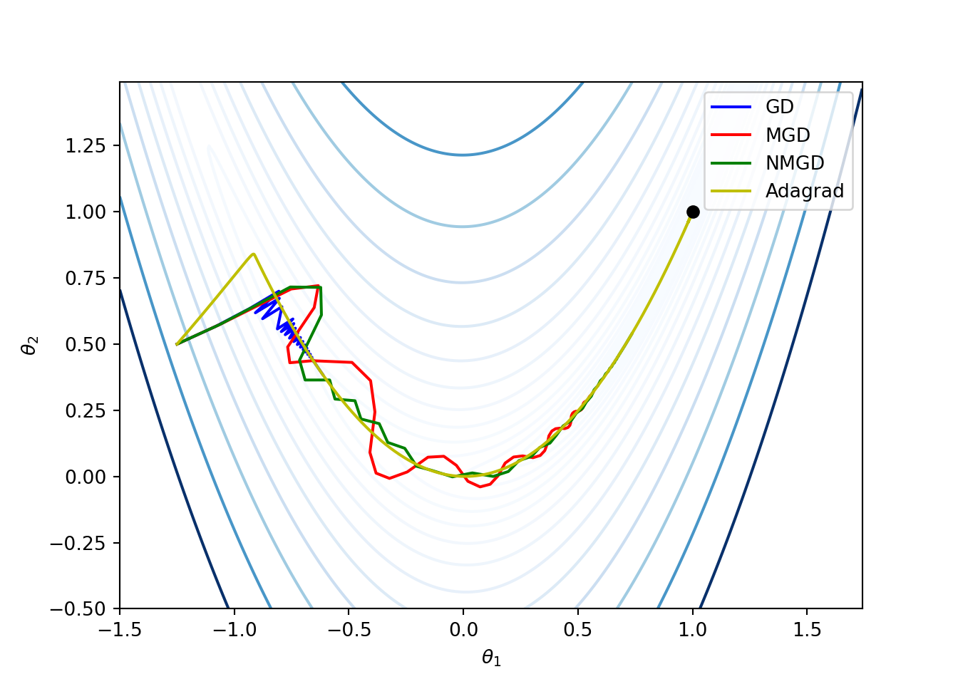
3.5.7 RMSprop
- RMSprop method comes from Lecture 6 of Geoff Hinton’s Coursera class.
Here, RMS stands for root mean square.
- RMSprop method overcomes the problem of monotonically decreasing learning rate by maintaining a decaying average of squared gradients. This average vector \(\widehat{\mathbf{S}}\) is updated according to \[ \mathbf s^{(k+1)} = \gamma_s {\mathbf s}^{(k)} + (1 - \gamma_s) \left(g^{(k)} \odot g^{(k)}\right), \] where \(\gamma_s\) is the decay factor, typically taken to be \(0.9\), and \(\odot\) denotes the element-wise product between vectors. Thus, the update of each element of \({\mathbf S}\) is given by \[\begin{equation} \tag{3.5} {s}_i^{(k+1)} = \gamma_s {s}_i^{(k)} + (1 - \gamma_s) \left(g_i^{(k)}\right)^2. \end{equation}\]
If the initial value \(\widehat{\mathbf S}^{(1)} = \mathbf 0\), then for each i, \[ {s}_i^{(k+1)} = (1 - \gamma_s)\sum_{j = 1}^k \gamma_s^{k - j}\left(g_i^{(j)} \right)^2. \]
Then the component-wise update of \(\theta\) is given by \[ \theta_i^{(k+1)} = \theta_i^{(k)} - \frac{\alpha}{\epsilon + \sqrt{{s}_i^{(k+1)}}} g_i^{(k)}, \] where the learning parameter is typically set to be \(0.001\).
The expression \(\sqrt{{S}_i^{(k+1)}}\) is called decaying root mean square of the time series \(g_i\), and is denoted by \(RMS(g_i)\). Then, \[ \theta_i^{(k+1)} = \theta_i^{(k)} - \frac{\alpha}{\epsilon + RMS(g_i)} g_i^{(k)}. \]
Exercise: Implement the RMSProp method for the Rosenbrock function considered earlier. Take \(\alpha = 0.01\), \(\gamma = 0.9\), and \(\epsilon = 10^{-8}\). Compare the performance with the adagrad method with \(\alpha = 0.01\) and \(\gamma = 0.9\).
3.5.8 Adadelta
Adadelta method is an extension of Agagrad method and it overcomes the problem of monotonically of the learning parameter.
The authors of RMSprop noticed that the units in gradient descent, stochastic gradient descent, momentum, Adagrad methods do not match. To fix this they use an exponentially decaying average of the squared updates as follows.
In addition to (3.5), let \(\widehat{\mathbf T}\) be the average vector updated according to \[ \widehat{T}_i^{(k+1)} = \gamma_t {\widehat T}_i^{(k)} + (1 - \gamma_t) \left(\Delta\theta_i^{(k+1)}\right)^2, \] for each component of \(\Delta \theta\), where \(\Delta \theta^{(k)} = \theta^{(k)} - \theta^{(k-1)}\), where \(\gamma_t\) is also decay parameter close to \(1\) and \(\widehat{T}^{(1)} = \mathbf 0\).
Then, in each iteration update the decaying average of the parameter vector by \[ \theta_i^{(k+1)} = \theta_i^{(k)} - \frac{\epsilon + RMS(\Delta \theta_i)}{\epsilon + RMS(g_i)} g_i^{(k)}, \] where \(RMS(\Delta \theta_i) = \sqrt{\widehat{T}_i^{(k)}}\).
The above expression eliminates the learning parameter completely.
3.5.9 Adam
The adaptive moment estimation, or simply adam, is a another method that adapts learning rates to each parameter \(\theta_i\).
In addition to using the exponentially decaying average of squared gradients (like RMSprop and Adadelta), the adam method also uses exponentially decaying average of gradients (like the momentum method).
Recall that the momentum method can be seen as a ball rolling down a slope. The adam method can be seen as a heavy ball with friction rolling down the slope.
The corresponding updates in each iteration of the adam method are: \[\begin{align*} \mathbf v^{(k+1)} &= \gamma_{v} \mathbf v^{(k)} + (1 - \gamma_v) g^{(k)},\\ \mathbf s^{(k+1)} &= \gamma_{s} \mathbf s^{(k)} + (1 - \gamma_s) \left(g^{(k)} \odot g^{(k)}\right). \end{align*}\]
\(\mathbf v^{(k)}\) and \(\mathbf s^{(k+1)}\) are estimates of the moment and the second moment of the gradient, respectively (hence the name of the method).
Since the initial values \(\mathbf v^{(1)} = \mathbf s^{(1)} = \mathbf 0\), the estimates \(\mathbf v^{(k)}\) and \(\mathbf s^{(k)}\) are biased towards zero, particularly when decay rates are small (i.e., \(\gamma_v\) and \(\gamma_s\) are close to 1).
Since \(\gamma_s\) and \(\gamma_v\) are close to \(1\), for small \(k\), \(\mathbf v^{(k)}\) and \(\mathbf s^{(k+1)}\) are biased towards \(\mathbf 0\). To eliminate this bias, the corrected (or unbiased) updates are \[\begin{align} \hat{\mathbf v}^{(k+1)} &= \frac{\mathbf v^{(k+1)}}{(1 - \gamma_v^k)},\\ \hat{\mathbf s}^{(k+1)} &= \frac{\mathbf s^{(k+1)}}{(1 - \gamma_s^k)} \end{align}\]
Finally, the parameter vector update is given by
\[ \theta^{(k+1)} = \theta^{(k)} - \alpha \frac{\hat{\mathbf v}^{(k+1)}}{\epsilon + \sqrt{\hat{\mathbf s}^{(k+1)}}}, \] where \(\epsilon\) is again on the order of \(1\times 10^{-8}\) to avoid division by zero.
The authors propose that a good default choice to be \(\gamma_v = 0.9\), \(\gamma_s = 0.999\), and \(\alpha = 0.001\).
3.5.10 Hypergradient Descent
The learning rate decides how sensitive the descent method to the gradient, and it has a substantial influence on the performance of the algorithm.
The accelerated descent methods presented above are either extremely sensitive to the learning rate or go to great extent to adapt the learning rate during execution.
The goal of the hypergradient methods is to use derivative of the learning rate parameter for improving the optimizer performance. This method applies gradient descent on the learning rate parameter.
The update of the learning parameter consists of the partial derivative of the objective function \(f\) with respect to the learning parameter: \[ \alpha^{(k+1)} = \alpha^{(k)} - \mu \frac{\partial f(\theta^{(k)})}{\partial \alpha}, \] where \(\mu\) is the hypergradient learning rate.
For gradient descent method, \[\begin{align*} \frac{\partial f(\theta^{(k)})}{\partial \alpha} &= \left(g^{(k)} \right) \boldsymbol{\cdot}\frac{\partial }{\partial \alpha}\left(\theta^{(k-1)} - \alpha g^{(k-1)}\right)\\ &= - g^{(k)} \boldsymbol{\cdot}g^{(k-1)} \end{align*}\]
Similarly, hypergradient descent idea can be applied to other gradient-based methods.
The key advantage of the hypergradient method is that it reduces the sensitivity of the algorithm to the hyperparameter.
3.6 Second-Order Methods
In the previous section on first-order methods, we used the gradient of the objective function \(f\) in the first-order approximation. In this section, we present some well-known methods that use second order approximations of \(f\).
3.6.1 Newton’s Method
As we have seen in the first-order methods, objective function value and its gradient help us in finding the direction of the next step. However, this information does not imply how far we need to travel.
On the other hand, Newton’s method uses a quadratic approximation of the objective function and finds the next step size by minimizing the quadratic function.
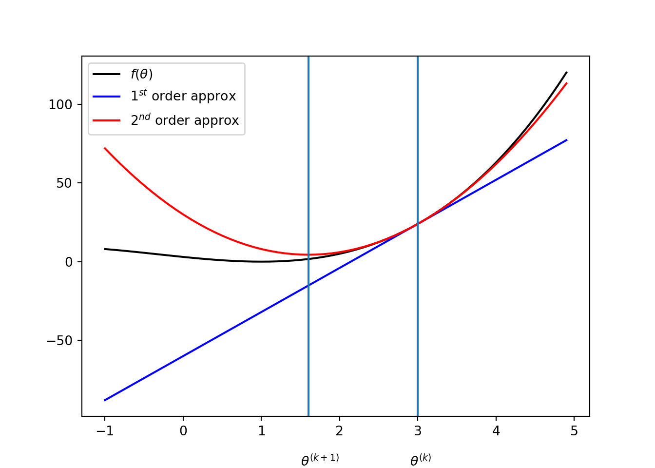
Consider the univariate case. In the \(k^{th}\) iteration, let \(q(x)\) be the quadratic approximation of the objective function \(f\) given by \[ f(\theta) \approx q(\theta) = f(\theta^{(k)}) + (\theta - \theta^{(k)}) f'(\theta^{(k)}) + \frac{(\theta - \theta^{(k)})^2}{2} f''(\theta^{(k)}). \]
Then the update is given by setting the derivative of \(q(x)\) to zero: \[ \frac{\partial}{\partial \theta} q(\theta) = f'(\theta^{(k)}) + (\theta - \theta^{(k)}) f''(\theta^{(k)}) = 0, \] then the solution is, \[ \theta^{(k+1)} = \theta^{(k)} - \frac{f'(\theta^{(k)})}{f''(\theta^{(k)})}. \] For instance, suppose that \(f(\theta) = (\theta - 1)^2(\theta + 3)\) and \(\theta^{(k)} = 3\). Then, \[ \theta^{(k + 1)} = 1.6. \]
For multivariate objective functions, update of Newton’s method is very similar to the univariate case: gradient replaces the derivative and Hessian replaces the second-order derivative. The quadratic approximation is given by \[ f(\theta) \approx q(\theta) = f(\theta^{(k)}) + (\theta - \theta^{(k)}) g^{(k)} + \frac{1}{2} (\theta - \theta^{(k)}) \boldsymbol{\cdot}\left(H^{(k)}(\theta^{(k)})(\theta - \theta^{(k)}) \right), \] where \(\nabla f(\theta^{(k)})\) and \(H^{(k)}\) are, respectively, the gradient and Hessian of \(f\) at \(\theta^{(k)}\). Then, the update can be obtained by taking gradient of \(q(\theta)\): \[ \nabla q(\theta) = g^{(k)} + H^{(k)}(\theta - \theta^{(k)}) = 0. \] Therefore, the update is given by \[ \theta^{(k+1)} = \theta^{(k)} - \left(H^{(k)} \right)^{-1}g^{(k)} \] given that \(H^{(k)}\) is non-singular (i.e., inverse exists).
Under certain conditions, the Newton’s method can exhibit a qudratic convergence, that is, there exists a constant \(c\) such that \[ \frac{\|\theta^{(k+1)} - \theta_\infty \|}{\|\theta^{(k)} - \theta_\infty \|^2} \leq c, \] for all \(k \geq 1\), where \(\theta_\infty\) is the limit of the sequence \(\theta^{(1)}, \theta^{(2)}, \dots\). In other words, the error in each iteration is proportional to the squared error of the previous iteration.
3.6.2 Instability of the Newton’s method
Update of \(\theta\) involves decision by the second derivative \(f''\). So, the update is undefined if \(f''(\theta^{(k)}) = 0\).
It can be instable when the second derivative \(f''(\theta^{(k)})\) is very close to zero, because then \(\theta^{(k+1)}\) can be too far from \(\theta^{(k)}\) to make the quadratic approximation invalid.
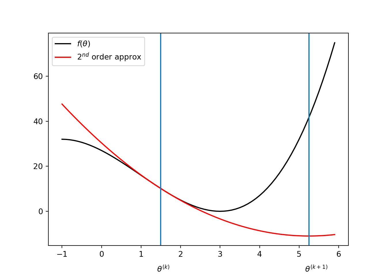
The following figures show situations where Newton’s method fail to work:
Overshoot: Consider \(f(\theta) = (\theta - 3)^2(t + 3)\) and \(\theta^{(k)} = 1.5\). Then, \(\theta^{(k +1 )} = 5.25\). It is clearly a overshoot.
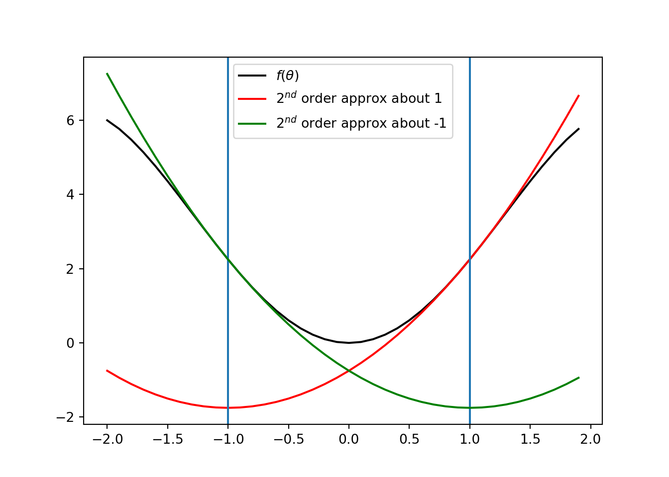
Oscillation: Consider \(f(\theta) = -\theta^4/4 + 5\theta^2/2\). If \(\theta^{(k)} = 1\), then we get \(\theta^{(k+1)} = -1\). That gives, \(\theta^{(k +2)} = 1\). So, the Newton’s methods continue to oscillate between \(-1\) and \(1\).
3.6.3 Secant Method
Consider the univariate case. Implementation of Newton’s method requires both the first derivative \(f'\) and the second derivative \(f''\). In many scenarios, we can have access to \(f'\), but not \(f''\).
The secant method is a modification of Newton’s method where the second derivative in each iteration is approximated by the last two iterations: \[ f''(\theta^{(k)}) \approx \frac{f'(\theta^{(k)}) - f'(\theta^{(k-1)})}{\theta^{(k)} - \theta^{(k-1)}}. \] That is, the updates in Secant method are given by \[ \theta^{(k+1)} = \theta^{(k)} - \frac{\theta^{(k)} - \theta^{(k-1)}}{f'(\theta^{(k)}) - f'(\theta^{(k-1)})} f'(\theta^{(k)}). \]
This method may take more iterations for convergence than Newton’s method and it also suffers from the problems associated with Newton’s method.
3.6.4 Quasi-Newton Methods
Consider multivariate cases where computing the inverse of Hessian is difficult or impossible.
As in the case of the secant method, quasi-Newton methods modifies the Newton’s method by approximating the inverse of Hessian.
The general update form the quasi-Newton methods is \[ \theta^{(k+1)} = \theta^{(k)} - \alpha^{(k)}Q^{(k)}g^{(k)}, \] where \(\alpha^{(k)}\) is scalar step factor and \(Q^{(k)}\) is an approximation of \(\left(H^{(k)} \right)^{-1}\) at \(\theta^{(k)}\). That is, the descent direction \(\mathbf d\) is given by \[ \mathbf d = - Q^{(k)}g^{(k)}.\]
Quasi-Newton methods typically starts with \(Q^{(1)}\) being the identity matrix.
To simplify the notation, define \[\begin{align*} \gamma^{(k+1)} &= g^{(k+1)} - g^{(k)}, \end{align*}\] and recall that \[\begin{align*} \Delta \theta^{(k+1)} &= \theta^{(k+1)} - \theta^{(k)} \end{align*}\]
We now discuss three quasi-Newton methods.
Davidon-Fletcher-Powell (DFP): This method uses the following update on \(Q\):
where \(^\top\) denotes the transpose operation.
-
The update of \(Q\) in (3.6) has the following properties:
If \(Q^{(1)}\) is symmetric and positive definite, \(Q^{(k)}\) is symmetric and positive definite in every iteration \(k\);
If \(f(\theta)\) has a quadratic form, that is, \[ f(\theta) = \frac{1}{2} \theta \boldsymbol{\cdot}A\theta + b \boldsymbol{\cdot}\theta + c, \] then \(Q = A^{-1}\). Thus, for this case, DFP and conjugate gradient methods have the same rate of convergence;
Storing and updating \(Q\) can be computationally demanding for high-dimensional problems, compared to conjugate gradient method;
Exercise: Prove properties (i) and (ii).
Broyden-Fletcher-Goldfarb-Shanno (BFGS): This method is an alternative to DFP method, and the update is as follows: \[\begin{align*} Q^{(k+1)} &= Q^{(k)} - \left(\frac{ \Delta\theta^{(k)} (\gamma^{(k)})^\top Q^{(k)} + Q^{(k)} \gamma^{(k)} (\Delta\theta^{(k)})^\top}{(\Delta\theta^{(k)})^\top \gamma^{(k)}}\right) \\ &\hspace{1.5cm}+ \left(1 + \frac{ (\gamma^{(k)})^\top Q^{(k)} \gamma^{(k)}}{(\Delta\theta^{(k)})^\top \gamma^{(k)}}\right)\frac{ \Delta\theta^{(k)} (\Delta \theta^{(k)})^\top}{(\Delta\theta^{(k)})^\top \gamma^{(k)}}. \end{align*}\] The BFGS is known to work better than the DFP method with approximate line search. However, storing \(n \times n\) matrix is challenging for higher dimensional problems.
Limited-memory BFGS (L-BFGS): To remedy the above issue with BFGS, limited memory BFGS (L-BFGS) approximates BFGS by storing the last \(m\) of \(\gamma\) and \(\Delta \theta\), rather than the storing the entire Hessian matrix.
In each iteration, the procedure has two steps to find the descent direction when current design point is \(\theta\).
First, backward procedure: Take \(\mathbf q^{(m)} = \nabla f(\theta)\), and define for each \(i = m-1, \dots, 1\) backward, \[\begin{equation*} \mathbf q^{(i)} = \mathbf q^{(i+1)} - \frac{\left(\Delta \theta^{(i+1)}\right)^\top \mathbf q^{(i + 1)}}{\left(\gamma^{(i+1)}\right)^\top \Delta \theta^{(i + 1)}} \gamma^{(i+1)}. \end{equation*}\] Then forward procedure: Take \[\mathbf z^{(0)} = \frac{\gamma^{(m)} \odot \Delta \theta^{(m)} \odot \mathbf q^{(m)}}{\left(\gamma^{(m)}\right)^\top \gamma^{(m)}},\] and define for \(i = 1, \dots, m\), \[\begin{equation*} \mathbf z^{(i)} = \mathbf z^{(i-1)} + \Delta \theta^{(i - 1)} \left( \frac{\left(\Delta \theta^{(i-1)}\right)^\top \mathbf q^{(i - 1)}}{\left(\gamma^{(i-1)}\right)^\top \Delta \theta^{(i - 1)}} - \frac{\left(\gamma^{(i-1)}\right)^\top \mathbf z^{(i - 1)}}{\left(\gamma^{(i-1)}\right)^\top \Delta \theta^{(i - 1)}}\right). \end{equation*}\] Finally, the descent direction is given by \[\mathbf d = - \mathbf z^{(m)}.\]
Exercise: Consider the Rosenbrock function mentioned earlier. Impliment and compare DFP, BFGS, and L_BFGS (with \(m = 3\)).
Page built: 2021-03-04 using R version 4.0.3 (2020-10-10)