Sequence Models have been motivated by the analysis of sequential data such text sentences, time-series and other discrete sequences data. These models are especially designed to handle sequential information while Convolutional Neural Network are more adapted for process spatial information.
The key point for sequence models is that the data we are processing are not anymore independently and identically distributed (i.i.d.) samples and the data carry some dependency due to the sequential order of the data.
Sequence Models is very popular for speech recognition, voice recognition, time series prediction, and natural language processing.
8.1 Learning outcomes
Sequence data
Recurrent Neural Network (RNN)
Long Short Term Memory (LSTM)
Transformers
Example: Usage of auto-encoders for language translation
8.2 Sequence data
Some applications includes:
Image Captioning: caption an image by analyzing the present action.
Figure 8.1: Neural Network Based Image Captioning source link
Machine Translation: Given an input in one language use sequence models to translate the input into different languages as output. Here a recent survey
RNN is especially designed to deal with sequential data which is not i.i.d.
RNN can tackle the following challenges from sequence data:
to deal with variable-length sequences
to maintain sequence order
to keep track of long-term dependencies
to share parameters across the sequence
8.3.1 Graphical Representation of RNN
The following figure exhibits the difference between the classical classic feed forward neural network architecture (left figure) and the Recurrent Neural Network:
Feed forward neural network also called vanilla neural network presents one input and provides one output without taking into account the sequence of the data.
Recurrent Neural Network introduce an internal loop wich allows information to be passed from one step of the network to the next. It apply a recurrence relation at every time step to process a sequence of data.
The unfold representation of the previous RNN is presented in the following figure which make more clear how the RNN can handle sequence data using the recurrence relation
\[\Large{\boxed{\underbrace{h^{<t>}}_{\textrm{cell state}} = f_W(\underbrace{h^{<t-1>}}_{\textrm{old state}}, \underbrace{x^{<t>}}_{\textrm{input vector}})}}\]
where \(f_W\) is a function parameterized by the weight \(W\). It is important to note that at every time step \(t\) the same function \(f_W\) is used and same set of weight parameters.
8.3.3 Weight Matrices parameters in RNN Sequence Modeling Tasks
Let introduce the weight parameters in the previous figure and precise some notation.
Below are the details associated with each parameter in the network.
\(x^{<1>}, \ldots, x^{<t-1>}, x^{<t>}, x^{<t+1>}, ... x^{<m>}\): the input data. In natural langage processing (NLP), for example, we can consider that the sequence input is a sentence of \(m\) words \(x^{<1>}, \ldots, x^{<t-1>}, x^{<t>}, x^{<t+1>}, ... x^{<m>}\).
\(x^{<t>} \in \mathbb{R}^{|V|}\): input vector at time \(t\). For example each word \(x^{<t>}\) in the sentence will be input as 1-hot vector of size \(|\mathcal{V}|\) (where \(\mathcal V\) is the vocabulary and \(|V|\) denotes the size).
\(h^{<t>} = \sigma(W_{hh} h^{<t-1>} + W_{hx} x^{<t>})\): the relationship to compute the hidden layer output features at each time-step \(t\).
\(\sigma(\cdot)\): the non-linearity function (sigmoid here)
\(W_{hx} \in \mathbb{R}^{D_h \times |\mathcal{V}| }\): weight matrix used to condition the input vector, \(x^{<t>}\). The number of neurons in each layer is \(D_h\)
\(W_{hh} \in \mathbb{R}^{D_h \times D_h}\): weights matrix used to condition the output of the previous time-step, \(h^{<t-1>}\)
\(h^{<t-1>} \in \mathbb{R}^{D_h}\): output of the non-linear function at the previous time-step, \(t-1\). \(h^{<0>} \in \mathbb{R}^{D_h}\) is an initialization vector for the hidden layer at time-step \(t = 0\).
Each desired output \(y^{<t>}\) is a 1-hot vector of size \(|\mathcal{V}|\) with 1 at index of \(x^{<t+1>}\) in \(\mathcal V\) and 0 elsewhere.
\(W_{yh} \in \in \mathbb{R}^{|\mathcal{V}| \times D_h}\): weights matrix used to compute the prediction at each time \(t\). For example, \(\hat{y}^{<t>} = softmax (W_{yh}h_t)\) and \(\hat{y} \in \mathbb{R}^{|\mathcal{V}|}\).
8.3.4 Different types of Sequence Modeling Tasks
Different tasks can be achieved using RNN:
Figure 8.9: Different types of Sequence Modeling Tasks source link
many-to-one: Sentiment Classification, action prediction (sequence of video -> action class)
one-to-many: Image captioning (image -> sequence of words)
many-to-many: Video Captioning (Sequance of video frames -> Caption)
many-to-many: Video Classification on frame level
8.3.5 How to train a RNN ?
RNN a clearly some nice features:
can process any length input
In theory for each time \(t\) can use information from many steps back
Same weights applied on every timestep
However RNN could be very slow to train and in practice it is difficult to access information from many steps back.
Let consider training a RNN for language model example:
We first have to get access to a big corpus of text which is a sequence of words \(x^{<1>}, \ldots, x^{<t-1>}, x^{<t>}, x^{<t+1>}, ... x^{<T>}\)
Forward pass into the RNN model and compute the output distribution \(\hat{y}^{<t>}\)
for every time \(t\) which represent the predict probability distribution of every word , given words so far
Compute the Loss fuction on each step \(t\). In this case the cross-entropy between predicted probability distribution \(\hat{y}^{<t>}\) and the true next word \(y^{<t>}\) (one-hot for \(\hat{x}^{<t+1>}\)):
Computiong the loss and the gradients accross entire corpus is too expensive. Then , in practice we use a batch of sentences to compute the loss and Stochastic Gradient Descent is exploited to compute the gradients for samll chunk of data, and then update.
8.3.6 Backpropagation through time
Let explicit the derivative of \(L\) w.r.t. the repeated weight matrix \(W_{hh}\).
Figure 8.10: Backpropagation through time source link
The backpropagation over time as two summations:
First summation over \(L\)
\[\Large{\boxed{
\frac{\partial L}{\partial W_{hh}}=\sum_{j=1}^{T} \frac{\partial L^{<j>}}{\partial W_{hh}}}}
\]
- Second summations showing that each \(L^{<t>}\) depends on the weight matrices before it:
\[\Large{\boxed{
\frac{\partial L^{<t>}}{\partial W_{hh}}=\sum_{i=1}^{t} \frac{\partial L^{<t>}}{\partial W_{hh}}}}
\]
Repeated matrix multiplication is required to get \(\dfrac{\partial h^{<t>}}{\partial h^{<k>}}\). It leads to a vanishing or exploding gradients issues.
8.3.7 Vanishing and Exploding gradient
Remind us that the RNN is based on this recursive relation
\[h^{<t>} = \sigma(W_{hh} h^{<t-1>} + W_{hx} x^{<t>}).\]
Let consider the identidy function \(\sigma(x)=x\), to help to understand why we have an issue with the computation of the gradient.
Let consider the gradient of the loss \(L^{<i>}\) on time \(i\), with respect to the hidden state \(h^{<j>}\) on some previous time \(j\) and denote \(\ell=i-j\). Then,
Then if \(W_{hh}\) is “small”, then this term gets exponentially problematic as \(\ell\) becomes large.
Indeed, if the weight matrix \(W_{hh}\) is diagonalizable:
\[W_{hh}=Q^{-1}\times \Delta \times Q,\]
where \(Q\) is composed of the eigenvectors and \(\Delta\) is a diagonal matrix with the eigenvalues on the diagonal. Computing the power of \(W_{hh}\) is then given by:
Thus eigenvalues lower than 1 will lead to vanishing gradient while eigenvalues greater than 1 will lead to exploding gradient.
8.3.8 Remarks
Note that gradient signal from faraway is lost because it’s much
smaller than gradient signal from close-by. Thus weights are updated only with respect to near
effects, not long-term effects. For example in langage modelling, the contribution of faraway words to predicting the next word at time-step \(t\) diminishes when the gradient vanishes early on.
The gradient can be viewed as a measure of the effect of the past on the future. Thus if gradient is small, the model cannot learn this dependency and the model unable to predict similar long-distance
dependencies at test time.
Exploding gradient is also a big issue for updating the weight and can cause too big step during the stochastic gradient descent. Moreover, once the gradient value grows extremely large, it causes an overflow (i.e. NaN).
A solution to solve the problem of exploding gradients has been first introduced by Thomas Mikolov who proposed the Gradient clipping. The principle is to scale down the gradient before applying an update when the norm of the gradient is greater than
some threshold.
8.4 Long Short Term Memory (LSTM)
LSTM is used to take into account long-term dependencies and was introduced by Hochreiter and Schmidhuber in 1997 to offer a solution to the vanishing gradients problem.
LSTM models make each node a more complex unit with gates controlling what information is passed through rather each node being just a simple RNN cell.
8.4.1 Main ideas
At each time \(t\), LSTM provides a hidden state (\(h^{(t)}\)) and a cell state (\(c^{(t)}\)) which are both vectors of length \(n\). The cell has the ability to stores long-tern information. Further, the LSTM model can erase, write and read information from the cell.
Gates are defined to get the ability to selection which information to either erased, written or read. The gates are also vectors of length \(n\). At each step \(t\) the gates can be open (1), closed (0) or somewhere in-between. Note that the gates are dynamic.
8.4.2 Graphical Representation of LSTM
Figure 8.11: Visual representation of LSTM source link
Figure 8.12: Understand LSTM respresentation source link
From a sequence of inputs \(x^{(t)}\), LSTM computes a sequence of hidden states
\(h^{(t)}\), and cell state \(c^{(t)}\):
Forget gate: controls what is kept versus forgotten, from previous cell state
Hidden state: read (“output”) some content from the cell
\[h^{(t)}=o^{(t)}\circ \textrm{tanh}\ c^{(t)} \]
8.4.3 Remarks
LSTM have been largely exploited for handwritting recognition, speech recognition, machine translation, parsing, image captioning.
The architecture of LSTM model is especially designed to preserve information over many timesteps. Indeed, LST maintains a separate cell state from what of outputted.
LSTM uses gates to control the flow of information
Backpropagating from \(c^{(t)}\) to \(c^{(t-1)}\) is only element-wise multiplication by the \(f\) gate, and there is no matrix multiplication by \(W\). The \(f\) gate is different at every time step, ranged between 0 and 1 due to sigmoid property, thus it overcome the issue of multiplying the same thing over and over again.
Backpropagating from \(h^{(t)}\) to \(h^{(t-1)}\) is going through only one single tanh nonlinearity rather than tanh for every single step.
The Backpropagation through time with uninterrupted gradient flow helps for the vanishing gradient issue even if LSTM does not guarantee vanishing/exploding gradient issues.
8.5 Gated Recurrent Units (GRU)
GRU has been proposed by Cho et al. in 2014 as an alternative to the LSTM.
For GRU model, there is no cell state and at each times step \(t\) there are an input \(x^{(t)}\) and hidden state \(h^{(t)}\).
Figure 8.13: Difference between LSTM and GRU source link
Update gate: controls what parts of hidden state are updated vs preserved
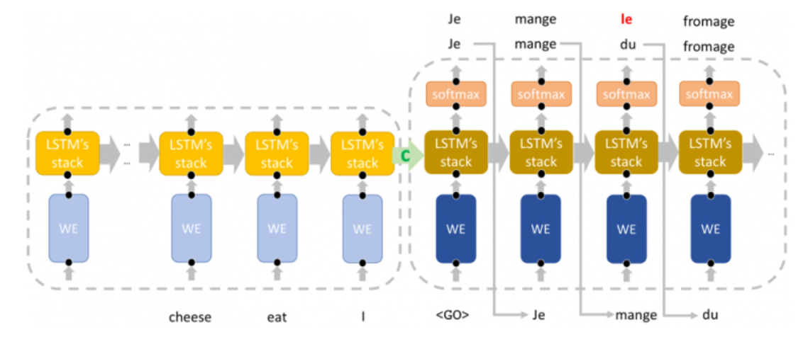
The encoder–decoder architecture has been introduced by Cho et al. (2014). A variant called sequence-to-sequence model has been introduced by Sutskever et al., (2014)
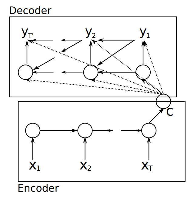
8.6.1 Cho’s model
Principle. In this model the encoder and decoder are both GRUs. The final state of the encoder is used as
the summary\(c\) and then this summary is accessed by all steps in the decoder
Figure 8.15: Cho’s model
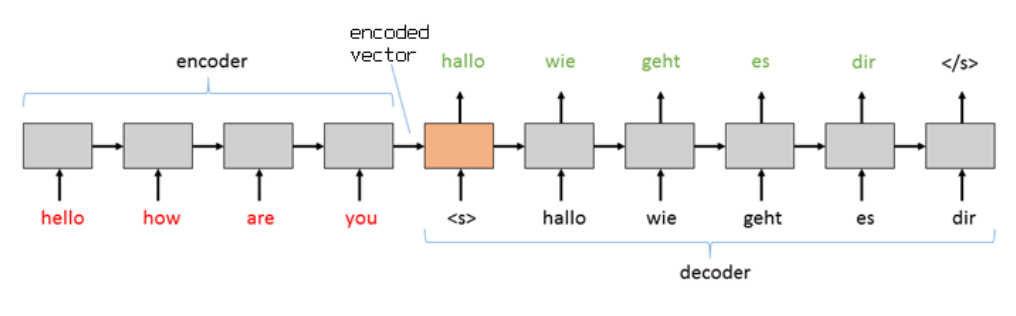
8.6.2 Sutskever’s model
Principle. In this model the encoder and decoder are multilayered LSTMs. The final state of the encoder becomes the initial state of the decoder. So the source sentence has to be reversed.
The main drawback of the previous models is that the encoded vector need to capture the entire phrase (sentence) and might skipped many important details. Moreover the information needs to “flow” through many RNN steps which is quite difficult for long sentence.
Figure 8.17: Limitation of Seq-to-Seq model
Bahdanau et al. (2015) have proposed to include attention layer which consist to include attention mechanisms to give more importance to some of the input words compared to others while translating the sentence.
Figure 8.18: The encoder-decoder model with additive attention (see Bahdanau et al. (2015))
A survey of the different implementations of attention model is presented by Galassi et al. (2019)
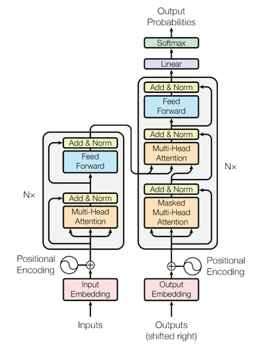
8.7 Transformer
Recently, Vaswani et al., 2017) offered a kind of revolution for Machine translation architecture:
“Attention is all you need”.
Figure 8.19: Transformer archichecture
This architecture is called the transformer which offers encoder-decoder structure that uses attention for information flow.
](images/image_caption.png)
](images/stock_price.png)
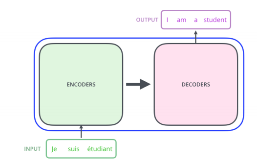 Figure 8.3: Machine translation
](images/speech_recognition.png)
](images/DNA_modelling.png) Figure 8.5: DNA sequence modelling
Figure 8.5: DNA sequence modelling ](images/intro_RNN.png)
](images/single_layer_RNN.png)
](images/multiple_layer_RNN.png) Figure 8.8: Multilayer Layer RNN
Figure 8.8: Multilayer Layer RNN 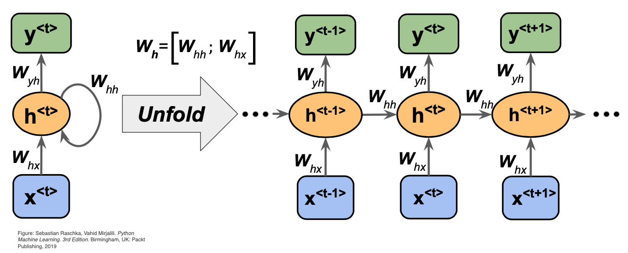
](images/type_sequence_Modeling.png)
](images/BTT_RNN.png)
](images/LSTM_gate_flow.png)
](images/LSTM_gate.png) Figure 8.12: Understand LSTM respresentation
Figure 8.12: Understand LSTM respresentation ](images/LSTM_GRU.png) Figure 8.13: Difference between LSTM and GRU
Figure 8.13: Difference between LSTM and GRU ](images/encoder-decoder.png)
)](images/encoder-decoder-attention.png)