See the latest book content here.
1 Supervised Machine Learning
Learning outcomes from this chapter:
- Forms of data: image data, tabular data, sequence data.
- The two forms of supervised learning: classification and regression.
- Hands on with basic classifiers: an ad-hoc classifier, least squares classifciation.
- Quantification of classification performance: accuracy, recall, and precision, F1 Score.
- Working with training, development and test sets.
- The concept of tuning hyper-parameters.
- The bias-variance tradeoff.
Source code for this unit is here.
1.1 A sea of data
Data is available in a variety of forms. This includes images, voice, text, tabular data, graphical data, and other forms.
In the typical case we consider a data point as a vector of length . Each coordinate of the vector is a feature. As there are multiple data points, say , we denote the data points as . We can then also consider the data as a matrix . This is a matrix with for and . Sometimes the transpose of the matrix is used. This transposed form is especially convenient if thinking of the data in tabular form such as a spreadsheet or data frame (each row is an observation and each column is a feature/variable).
Note that an alternative to the data being of the form is sequence data where and the data sequence can essentially continue without bound. Such sequence data is typical for text, voice, or movies. We handle such cases in Unit 8 – Sequence Models.
1.1.1 Forms of the datapoint
A data point can be quite a complicated object, such as an image, or even a movie. In such a case, we can stil vectorize the data to represent it in a vector. The exact interpretation of the data varies. Here are some examples:
Voice recording: Here a simple representation is the amplitude of the recording at regular intervals, say every seconds (every micro seconds) when recording at samples per second. The amplitude can be a positive or negative number, sometimes defined over a finite range (e.g. only one of values if each sample is a single byte). Hence for example a voice recording of an English sentence of seconds will be a vector with entries (features).
A monochrome image: Here consider an image of by pixels with each pixel signifying the intensity e.g. is black and (or some other maximal value) is white. We can consider the image as a matrix and the vector of length as a vectorized formed of the matrix. That is if we consider column-major vectorization then for any , we set and Similarly with row-major vectorization we set and As an example consider a (portrait) image. In this case features (pixels).
A color image: Here each pixel is not just an intensity but rather an RGB (Red, Green, Blue) -tuple. One way to represent this image is in the -tensor which is dimensional. Again, similarly to the case of a monochrome image it is possible to vectorize the image to a dimensional vector with . An image of the same dimensions as before has features. Note that if considering say values for each color component then then each feature is represented by bytes and the memory size of is bytes which is roughly Megabytes (a Megabyte is typically considered to be bytes which is only approximately ). In practice, images are often stored in a much more compressed format - although for deep learning purpuses they are often expanded to this type of bitmap format.
A (silent) color movie: Here there is another dimension which is the number of frames in the movie and each frame is an image. Hence the movie is a -tensor of dimensions . It can also (in principle) be vectorized into a vector . To get a feel for the dimension (number of features) in assume it is a high quality movie as before with each image (frame) having features. If the movie has 30 frames per second and spans minutes then it is composed of images, so the total number of features is . This would take about Gigabytes in such raw form. Note that in practice movies are stored in compressed formats.
A text corpus: Text written in ASCII, Unicode, or other means is collection of characters. One way to consider text is as sequence data (similarly this can be done for voice recordings and movies). An alternative way is to summarize the text into a word frequency histogram where a collection of words in the dictionary, say words are mapped to the entries of the vector . Then is the frequency of how many times the word appeared in the text. Wit such a representation, it is quite clear that for non-huge texts is a sparse vector.
Hetorgenous datasets: In many cases the features for a certain observation/data-point/individual are very hetorgenous. This is for the example the case coming from survey data, or other personal data where each feature (or subset of features) is completely different from the rest. This is the type of information appearing in a data frame. Features can be categorical (in which case we can encode them numerically) or numerical.
An alternative phrase common in statistics is the response variable. The labels: When dealing with supervised learning, each data point also has a label (or response variable). This is denoted as . In classification problems there is a finite set of values which the label can take, which we consider as without loss of generality. In regression problems the labels are real-valued.
1.1.2 Popular (example) datasets
Here are a few popular datasets:
- Boston Housing Prices Dataset
- Iris Dataset
- [Wisconsin Breast Cancer Dataset](https://archive.ics.uci.edu/ml/datasets/Breast+Cancer+Wisconsin+(Diagnostic)
- MNIST
- Fashion MNIST
- CIFAR-10
- ImageNet
- YouTube-8M
- Twitter Sentiment Analysis
- 20 Newsgroups
- A sound vocabulary and dataset
And here is a nice video describing a few of these:
See also:
1.1.3 The MNIST dataset
One of the most basic machine learning datasets is MNIST. In this case, each is a black and white image of a digit, and when vectorized is a long vector. Each label is an element from indicating the real meaning of the digit. The dataset is broken into a training set involving images, and a testing set involving an additional images. Hence in total .
 Figure 1.1: The first image in the MNIST training set. Clearly for this image.
We use this example to also deviate momentarily from supervised learning for some exploratory data anslysis (EDA) as well as a bit of unsupervised learning.
Here as an example is the first image. Pixels have values in the range with being “fully off” (black in this representation) and 1.0 being “fully on”.
And here are the first 30 images
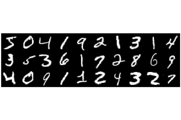 Figure 1.2: The first 30 MNIST images
#Julia code
using Plots, Flux.Data.MNIST; pyplot()
imgs = MNIST.images()
heatmap(vcat(hcat(imgs[1:10]...),
             hcat(imgs[11:20]...),
             hcat(imgs[21:30]...)),ticks=false)
The proportion of 0 pixels is about 80%, and within the non-zero pixels, the mean intensity is about . The proportion of pixels that are fully saturated () is 0.00668. As presented below, label counts are approximately even among labels, hence this is a balanced dataset. We also plot density plots of the distribution of the number of pixels that are on, per digit.
![]() Figure 1.3: The distribution of the number of on-pixels per digit label
Figure 1.3: The distribution of the number of on-pixels per digit label
#Basic Exploratory Data Analysis (EDA) for MNIST with Julia
using Statistics, StatsPlots, Plots, Flux.Data.MNIST; pyplot()

imgs, labels   = MNIST.images(), MNIST.labels()
x = hcat([vcat(float.(im)...) for im in imgs]...)

d, n = size(x)
@show (d,n)

onMeanIntensity = mean(filter((u)->u>0,x))
@show onMeanIntensity

prop0 = sum(x .== 0)/(d*n)
@show prop0

prop1 = sum(x .== 1)/(d*n)
@show prop1

print("Label counts: ", [sum(labels .== k) for k in 0:9])

p = plot()
for k in 0:9
    onPixels = [ sum(x[:,i] .> 0) for i in (1:n)[labels .== k] ]
    p = density!(onPixels, label = "Digit $(k)")
end
plot(p,xlabel="Number of non-zero pixels", ylabel = "Density")```
(d, n) = (784, 60000)

onMeanIntensity = 0.6833624860322157

prop0 = 0.8087977040816327

prop1 = 0.006681164965986395

Label counts: [5923, 6742, 5958, 6131, 5842, 5421, 5918, 6265, 5851, 5949]
We can also carry out Principal Component Analysis (PCA) for the whole dataset. We won’t cover PCA here, but this video may be useful.
When we carry out PCA and then plot each image based on the first two principle components, we get the following (this example is taken from here:
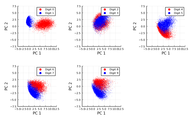 Figure 1.4: Basic Principal Component Analysis (PCA) for MNIST
#Julia code
using MultivariateStats,LinearAlgebra,Flux.Data.MNIST,Measures,Plots
pyplot()

imgs, labels   = MNIST.images(), MNIST.labels()
x = hcat([vcat(float.(im)...) for im in imgs]...)
pca = fit(PCA, x; maxoutdim=2)
M = projection(pca)

function compareDigits(dA,dB)
    imA, imB = imgs[labels .== dA], imgs[labels .== dB]
    xA = hcat([vcat(float.(im)...) for im in imA]...)
    xB = hcat([vcat(float.(im)...) for im in imB]...)
    zA, zB = M'*xA, M'*xB
    default(ms=0.8, msw=0, xlims=(-5,12.5), ylims=(-7.5,7.5),
            legend = :topright, xlabel="PC 1", ylabel="PC 2")
    scatter(zA[1,:],zA[2,:], c=:red,  label="Digit $(dA)")
    scatter!(zB[1,:],zB[2,:], c=:blue, label="Digit $(dB)")
end

plots = []
for k in 1:5
    push!(plots,compareDigits(2k-2,2k-1))
end
plot(plots...,size = (800, 500), margin = 5mm)
We can also carry out k-means clusterming for the whole dataset with . When we do this we get centroids of the 10 clusters that resemble smoothed digits. This type of clustering algorithm works by iterating two steps: (1) Finding centers (sometimes called centroides) of the currently specified clusters. And (2) assigning the clusters based on the current centers. It is very simple. Here is a video that shows it for with and a specification of four clusters:
And here it is done for the MNIST dataset with the number of clusters naturally specified as .
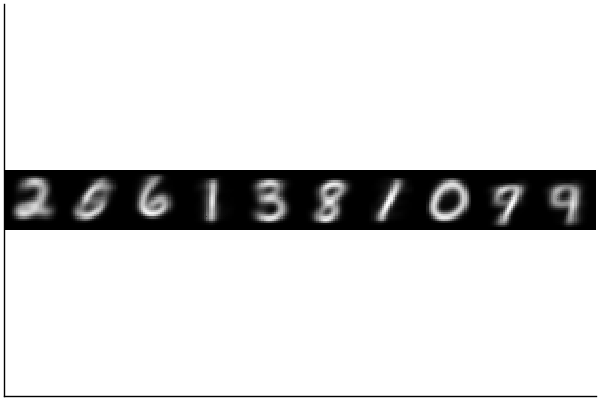 Figure 1.5: MNIST clustering - the centroids
#Julia code
using Clustering, Plots, Flux.Data.MNIST, Random; pyplot()
Random.seed!(0)
imgs, labels   = MNIST.images(), MNIST.labels()
x = hcat([vcat(Float32.(im)...) for im in imgs]...)
clusterResult = kmeans(x,10)
heatmap(hcat([reshape(clusterResult.centers[:,k],28,28) for k in 1:10]...),
    yflip=true,legend=false,aspectratio = 1,ticks=false,c=cgrad([:black, :white]))
It is then interesting to look at the centers (centroids). None of them are any specific real image but they are rather the average image of each cluster.
1.2 Classification and Regression Problems
In supervised learning we wish to find a model which takes in a data point and computes an estimated label. In case of regression, labels are continuous variables and we can view the model as . In case of classification the labels fall in some finite set and we can view the model as .
1.2.1 Classification
Training of a supervised learning classification algorithm is the process of considering the data to produce a classifier . Common algorithms include the support vector machine (SVM), random forest, and naive Bayes estimation. However our focus in this course is almost entirely on deep learning of which the perceptron, logistic regression, and softmax regression are basic examples, and convolutional deep neural networks are more involved examples.
In the case of a dataset like MNIST, a classifier , is a function from the input image (vector) in to the set of labels where and the actual meaning of label is the digit . Since we say that such a classification problem is a multi-class problem, but in cases where the problem is a binary classification problem. One may consider for example a relabeling of the labels in MNIST where every digit that is not the -digit is labeled as (negative) and all the digits that are digits are labeled as (positive). Such a binary classification would aim to find a classifier that distinguishes between digits that are not and digits that are .
Note that often, we can use a collection of binary classifiers to create a multi-class classifier. For example, assume we had a binary classifier for each digit (indicating if is positive meaning it is from digit or negative meaning it is not from digit ). Assume further that when we classify we actually get a measure of the certainty of the sample being positive or negative, meaning that if that measure is a large positive value we have high certainty it is positive, if it is a small positive value we have low certainty, and similarly with negative values. Denote this measure via . We can then create a multi-class classifier via,
This type of strategy is called the one-vs-rest (or one-vs-all) strategy as it splits a multi-class classification into one binary classification problem per class and then chooses the most sensible class. Note that an alternative is called the one-vs-one strategy in which case for each digit we would create classification problems to distinguish between all other digits. We can denote these classifiers by for distinguishing between digits and (and note that is the same classifier). Then there are a total of such classifiers. If similarly we have certainty measures then the overall multiclass classifier can be constructed via
1.2.2 Regression
In a case of a dataset like MNIST regression is not typically relevant. However assume hypothetically that there was another type of label associated with the dataset, indicating the duration it took to hand write each digit (say measured in milliseconds). We would still denote these labels via only this time they would be real valued. Now a model is not called a classifier but rather predictor as it takes an image and indicates an estimate of the duration of time it took to write the label.
1.2.3 Applications of classification
Some of the biggest successes of Deep Learning in the past decade have been with regards to image classification. For example, lets try to use a famous pretrained network, VGG19, to classify this image,
Here we use the Metalhead.jl Julia package as a wrapper for the VGG19 pre-trained model. We’ll study more about neural network models such as this in the course, but for now think of the (pre-trained) neural network as a function . This apple image isn’t exactly so a “wrapper” will translate the image into that format. VGG determines the image to be one of a thousand labels.
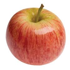 Figure 1.6: An image of an apple
 Figure 1.7: An image of a baby
#Julia code
using Metalhead

#downloads about 0.5Gb of a pretrained neural network from the web
vgg = VGG19();
vgg.layers

#download an arbitrary image and try to classify it
download("https://deeplearningmath.org/data/images/appleFruit.jpg","appleFruit.jpg");
img = load("appleFruit.jpg");
classify(vgg,img)

#and again
download("https://deeplearningmath.org/data/images/baby.jpg","baby.jpg");
img = load("baby.jpg");
classify(vgg,img)
"Granny Smith"
"diaper, nappy, napkin"
The output “Granny Smith” is correct in this case, but when we try for this image we got “diaper, nappy, napkin”, which is maybe somewhat close but not exactly correct.
1.2.4 Applications of regression
As a simple example consider a uni-variate feature indicating the square footage (area) of a house, and as the selling price. In this case simple linear regression, can work well to find a line of best fit and even provide confidence bands around the line if we are willing to make (standard) statistical assumptions about the noise component .
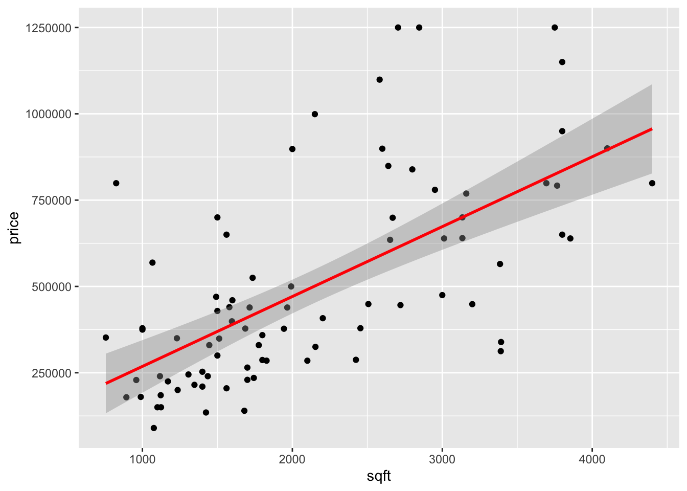 Figure 1.8: House price prediction
#R Code
library(ggplot2)
load("house_data.RData")
p1 <- ggplot(house, aes(sqft, price)) +
  geom_point() + stat_smooth(method = "lm", col = "red") +
  xlab("sqft") + ylab("price")+
  theme(legend.position = 'bottom')
p1
In other cases a simple linear model doesn’t work well and we can create additional features out of . For example a new feature is and then we can fit the model,
# Load the data
library(MASS)
library(tidyverse)
library(caret)
data("Boston", package = "MASS")
# Split the data into training and test set
set.seed(123)
training.samples <- Boston$medv %>%
  createDataPartition(p = 0.8, list = FALSE)
train.data  <- Boston[training.samples, ]
test.data <- Boston[-training.samples, ]
model.lm <- lm(medv~lstat,data=train.data)
model.quad <- lm(medv~lstat+I(lstat^2),data=train.data)
RMSE.train <- sqrt(mean((train.data$medv-predict(model.lm))**2))
RMSE.test <- sqrt(mean((test.data$medv-predict(model.lm,newdata=test.data))**2))
#RMSE.train
#RMSE.test
RMSE.train.quad <- sqrt(mean((train.data$medv-predict(model.quad))**2))
RMSE.test.quad <- sqrt(mean((test.data$medv-predict(model.quad,newdata=test.data))**2))
#RMSE.train.quad
#RMSE.test.quad
tab <- data.frame("Model"=c("linear","quadratic"),"Train"=c(RMSE.train,RMSE.train.quad),"Test"=c(RMSE.test,RMSE.test.quad))
knitr::kable(tab,caption="Root Mean Squared Error",digits = 2)
Table 1.1: Root Mean Squared Error
| Model | Train | Test |
|---|---|---|
| linear | 6.13 | 6.50 |
| quadratic | 5.48 | 5.63 |
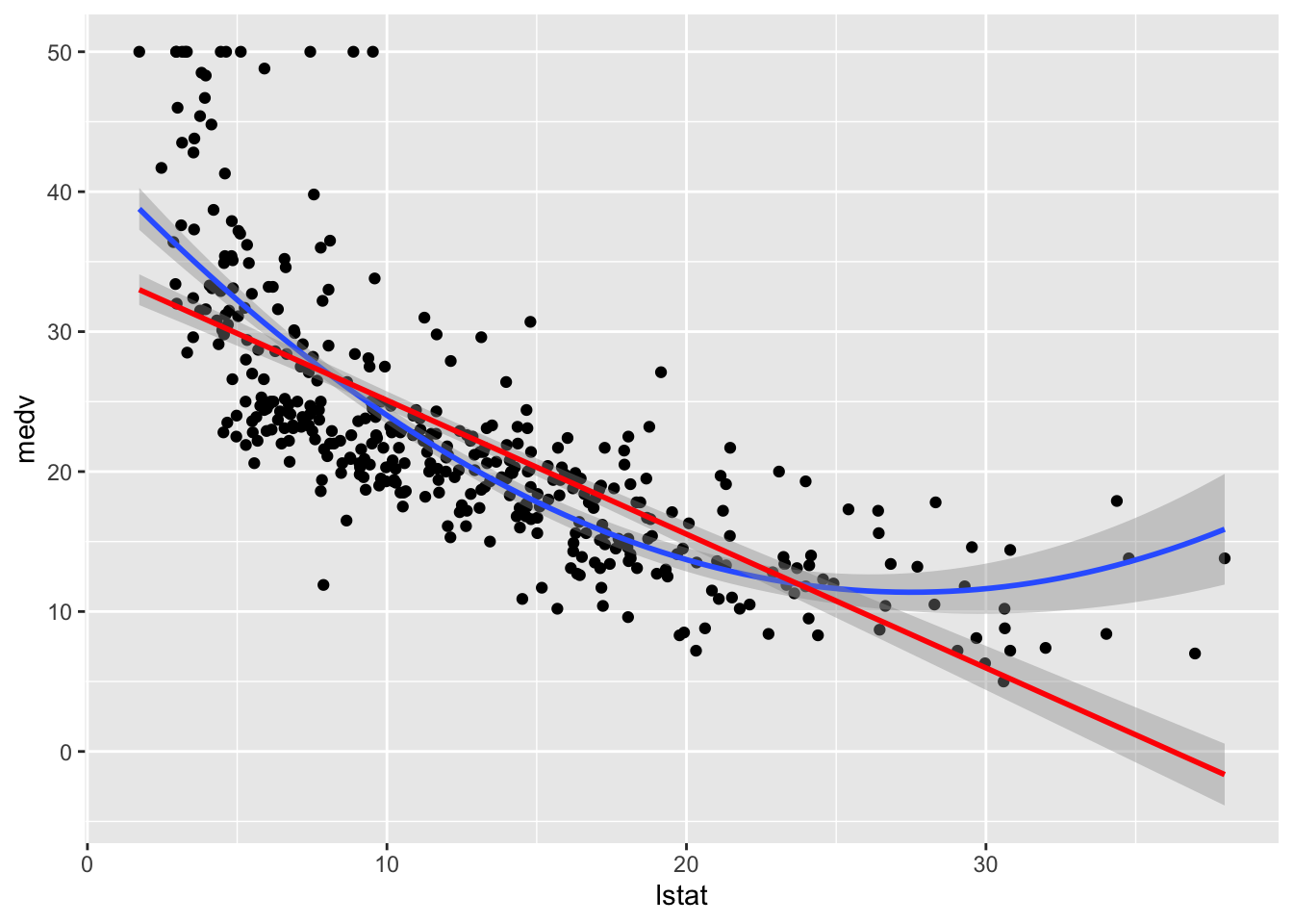 Figure 1.9: House price prediction (in Boston Suburbs)
ggplot(train.data, aes(lstat, medv) ) +
  geom_point() +
  stat_smooth(method = lm, formula = y ~ poly(x, 2, raw = TRUE))+
  stat_smooth(method = lm, formula = y ~ x,col='red')
These are classic applications of regression for which statistical practice and tradition is well suited. Model based fitting of linear models, generalized linear models, and other generalizations is now common practice and is a basic tool in the toolset of the statistican and data-scientist.
1.2.4.1 A second example
For this we consider the Safe Blues project. This experimental project deals with online measurements of a virtual safe epidemics. These virtual safe virus-like tokens are spread via cellular phones. The idea is then to exploit the fact that the virtual epidemic has some correlation to actual epidemic spread. In this simulation figure, a biological epidemic in red is observed during days 1-100. During that time, and also up to day 115, multiple Safe Blues (virtual) epidemics are observed. The virtual epidemics behave somewhat like the biological epidemic because the physical interactions that occur between people also (roughly) occur between their cellular phones.
The figure below presents a simulated (biological) epidemic in red, together with multiple simulated Safe Blues strands in thin blue.
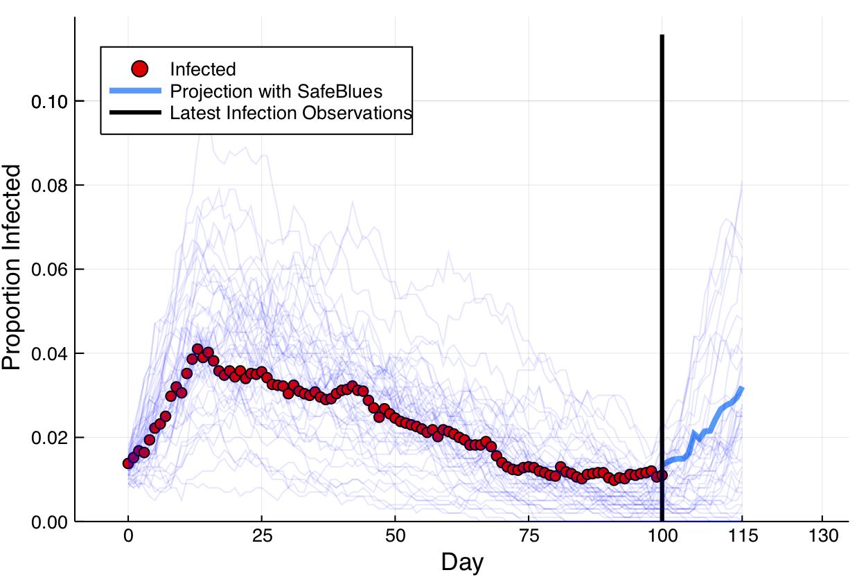
Safe Blues strands in light blue behave somewhat like a real epidemic but can be measured in real-time.
A (relativly simple) neural network model relates the state of all Safe Blues strands to the state of the biological virus. This model is trained at day 100, after 100 days of measurments of Safe Blues strands (). Call the model . Then during days the on line Safe Blues strand measurments are used with to predict the level of the actual epidemic. This creates the blue curve.
This video explains a bit more:
1.3 The Train, Dev, Test workflow
The typical scenario in supervised learning is to use data to train a classifier on seen data and then use the classifier later on unseen data. For example with digit classification we can use the MNIST dataset to obtain a good classifier and then later, when presented with an unseen datapoint (image) for which we don’t know the label , we can use as our best guess of the (never to be seen) label .
With such a process the underlying assumption is that the nature of the seen data is similar to the unseen data. Proper sampling is often needed for this.
The process of developing the classifier called learning and the usage of the classifier as part of a technological solutions such as apps or scientific modeling is sometimes called production. In more advanced scenarios active learning is used and the processes of learning and production are merged. We won’t deal much with active learning in this course.
The learning process is generally broken up into the acts of training, validation, and testing. In general, the training phase implies adjusting parameters of so that it predicts the data best. Further the validation phase implies adjusting hyper-parameters associated with or the training process itself. In practice, the training and validation phases are often mixed in the sense that we train, then validate, adjust parameters, train again, etc.
The testing phase implies simulating a production scenario using the seen data and checking how well the classifier or predictor works on that data. In general, testing should only be carried out once because going back and readjusting the classifier after testing will violate the validity of the test.
Before starting learning, we break the seen data into three different data chunks. The train set, the validation set, and the test set. The train set is the main dataset used to calibrate the learned parameters of . The validation set is used to adjust hyper-parameters (including model selection) before repeating training with the train set. Finally, once a final model is chosen, it is evaluated on the test set. This application on the test set is used to given an indication of how well the classifier or predictor will work in production, on unseen data.
1.4 Example classifiers and performance measures
We now take a step back from the advanced neural network models and applications and explore few basic classifiers. As we do so we see different ways of determining the performance of the the model as well as basic notions of loss functions, optimization, and iterative training.
1.4.1 An AdHoc classifier for 1 digits
Deep learning and other general machine learning methods in this chapter are general and work well on a variety of datasets. Such generality is useful as it relieves one from having to custom fit the machine learning model to the exact nature of the problem at hand. Nevertheless as a vehicle for illustration of the aforementioned concepts of binary classification, we now present a model that is only suited for a specific problem. Note that even for the specific problem. This is for illustrative purposes.
With the MNIST data we only wish to classify if an image is the digit or not. How would we do that? Here we go for a direct method related to the way in which digits are drawn. We rely on the fact that digits roughly appear as a vertical line while other digits have more lit up pixels not just on a vertical line within the image. This is clearly only a rough description because the character involves more than just a vertical line.
With this observation, our classifier works by considering each of the rows of the image and locating the maximal (brightest) pixel out of the pixels in that row. We reason that if the image is a digit, then on each row, there will generally only be a few neighboring bright pixels to the maximal pixel. However, if it is not a digit, there may potentially be other bright pixels on the row. For this we include two pixels to the left of the brightest pixels and two pixels to the right as long as we don’t overshoot the boundary. We then sum up these pixels and do so for every row. Finally we divide this total by the total sum of the pixels and call this function the peak proportion and represent it via,
We may expect that for images representing a digit, the peak proportion is high (close to unity), while for other images it isn’t. This is indeed the case as presented on the left of the following figure. The plot presents the distribution of the peak proportion value when considering images in the MNIST train set. The (Julia) source that creates this Figure is here
See the source code here.
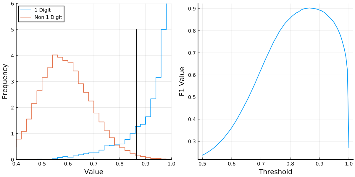 We thus see that is a sensible statistic to consider because it allows to seperate positive samples from negative samples. Note that such separation would be useless when trying to compare other digits, as it is tailor made for the digit .
A question is now how to choose a threshold parameter, where the classifier is
In this case is the parameter and in the training process we optimize the parameter . Clearly if is very low (near 0) almost every digit would be classified as a 1 digit, whereas if is high (near 1) almost every digit would be classified as a negative (or a 0 digit).
The question is now how to determine the “best value” of and prior to that to define a suitable performance measure under which “best value”.
1.4.2 Accuracy
When considering a classifier , the most basic way to quantify the performance is via the accuracy. Given feature data and labels , which is either the training set, validation set, or test set, the accuracy is the proportion of labels that are correctly predicted. Namely,
In many cases this is a very sensible measure. However when dealing with unbalanced data (where some labels are much more common than others), considering accuracy on its own is not enough.
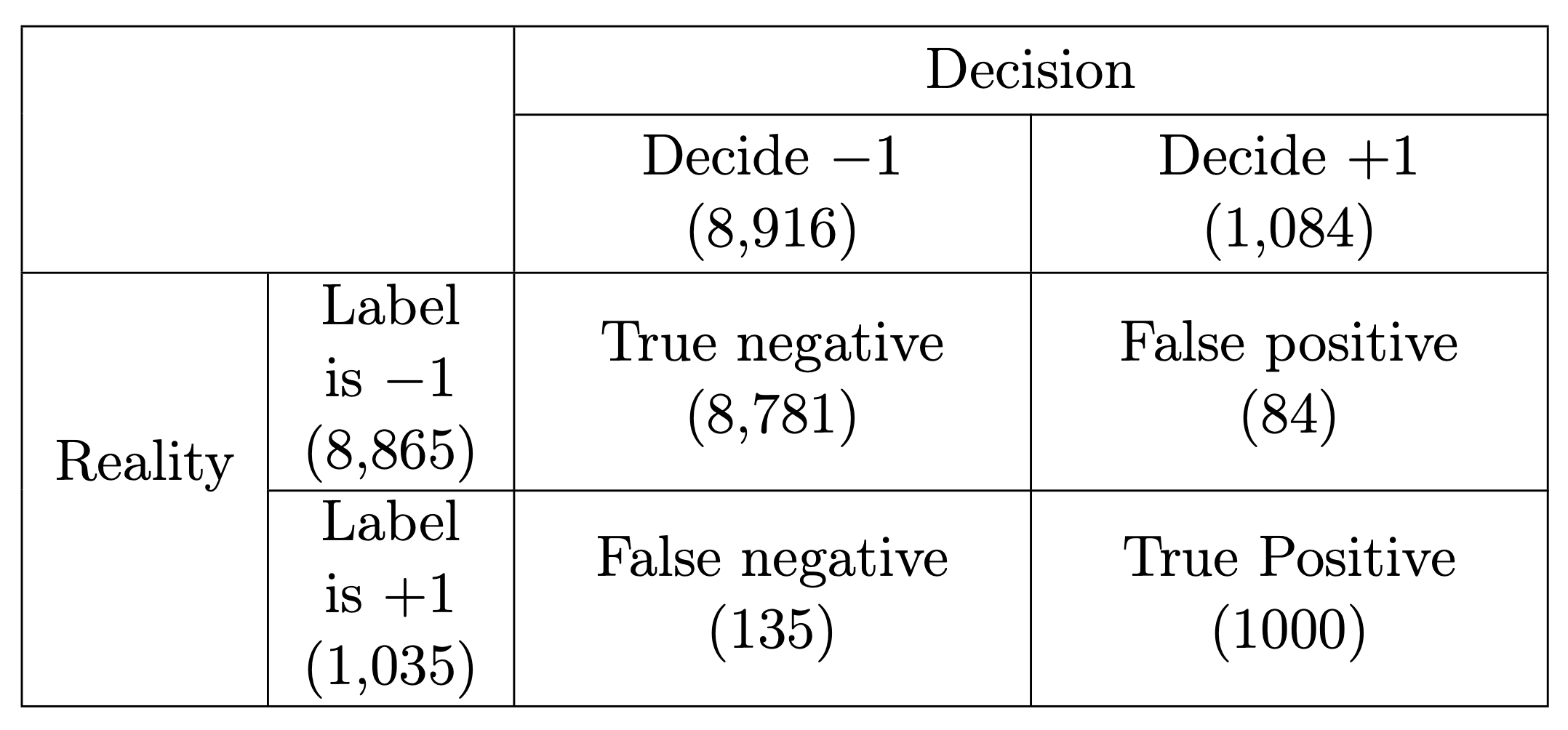
For example, if we return to the goal of classifying if an MNIST digit is (positive) or not (negative), then out of the test set of images there are positive samples and the remaining samples are negative. Hence a degenerate classifier such as would achieve a accuracy of almost . This might sound good, but it is clearly not a valid measure of the quality of estimator in such a case.
1.4.3 Precision and Recall
It is common to use the pair of performance measures, precision and recall which we describe below.
Comparing with classical statistics, observe that the recall is essentially equivalent to the power of a statistical test as it quantifies the chance of detecting a positive in case the label is actually positive. This is also called sensitivity in biostatistics. However the precision does not agree with the specificity from biostatistics (or as denoted in statistical tests). Nevertheless, a high precision implies a low rate of false positives similarly to the fact that in statistical testing, a high value (or specificity) also means a low number of false positives.
It is clear that ideally we wish the classifier to have as few false positives and false negatives as possible, but these are often competing objectives. Precision and recall help to quantify these objectives and are computed as follows where stands for the number of elements in a set.
In our case:
The closer we are to , the better.
In designing classifiers, precision and recall often yield competing objectives where we can often tune parameters and improve one of the measures at the expense of the other. In the context of (classical) statistical testing, things are more prescribed since we fix , the probability of Type I error, at an accepted level (e.g. ), and then search for a test that minimizes , the probability of Type II error (this is maximization of power, sensitivity, or recall). However in machine learning, there is more freedom. We don’t necessarily discriminate between the cost of false positives and false negatives, and even if we do, it can be by considering the application at hand.
1.4.4 Averaging Precision and Recall: The score
A popular way to average precision and recall. is by considering their harmonic mean of the two. This is called the F score and is computed as follows: In our example, . Here is a blog post descrbing the arithmetic, geometric, and harmonic means. While we don’t cover it further, we note that sometimes you can use a generalization of called the where determines how much more important is recall in comparison to precision (do not confuse with of hypothesis testing). However in general, if there is not a clear reason to price false positives and false negatives differently, using the score as a single measure of performance is sensible.
We do this by plotting the score as a function of and choosing the optimal which turns out to be . This then yields the classifier.
1.4.5 Linear classifiers
The previous classifier may be somewhat useful for determining if a digit is 1 or not, however the idea isn’t easily extended to other digits or other types of data. For this machine learning seeks to find generic algorithms that do not directly rely on the nature of the data at hand. One of the simplest such algorithms is simply the linear classifier which uses least squares.
We consider each image as a vector and obtain different least squares estimators for each type of digit using a one vs. rest approach. For digit we collect all the training data vectors, with . Then for each such , we set and for all other with , we set . This labels our data as classifying “yes digit ” vs. “not digit ”. Call this vector of and values for every digit . We compute, where is the dimensional pseudo-inverse associated with the (training) images. It is the pseudo-inverse of the matrix (allowing also a first column of ’s for a bias term). The matrix is constructed with a first column of ’s, the second column having the first pixel of each image, the third column having the second pixel of each image, up to the last column having the ’th pixel of each image. The pixel order is not really important and can be row major, column major, or any other order, as long as it is consistent.
Now for every image , the inner product of with the image (augmented with a for the constant term) yields an estimate of how likely this image is for the digit . A very high value indicates a high likelihood and a low value is a low likelihood. We then classify an arbitrary image by selecting,
Observe that during training, this classifier only requires calculating the pseudo-inverse of once as it is the for all digits.
It then only needs to remember vectors of length , . Then based on these vectors, a decision rule is very simple to execute.
This example is taken from here
using Flux, Flux.Data.MNIST, LinearAlgebra
using Flux: onehotbatch

imgs   = Flux.Data.MNIST.images()
labels = Flux.Data.MNIST.labels()
nTrain = length(imgs)
trainData = vcat([hcat(float.(imgs[i])...) for i in 1:nTrain]...)
trainLabels = labels[1:nTrain]
testImgs = Flux.Data.MNIST.images(:test)
testLabels = Flux.Data.MNIST.labels(:test)
nTest = length(testImgs)
testData = vcat([hcat(float.(testImgs[i])...) for i in 1:nTest]...)

A = [ones(nTrain) trainData]
Adag = pinv(A)
tfPM(x) = x ? +1 : -1
yDat(k) = tfPM.(onehotbatch(trainLabels,0:9)'[:,k+1])
bets = [Adag*yDat(k) for k in 0:9]

classify(input) = findmax([([1 ; input])'*bets[k] for k in 1:10])[2]-1

predictions = [classify(testData[k,:]) for k in 1:nTest]
confusionMatrix = [sum((predictions .== i) .& (testLabels .== j))
                for i in 0:9, j in 0:9]
accuracy = sum(diag(confusionMatrix))/nTest

println("Accuracy: ", accuracy, "\nConfusion Matrix:")
show(stdout, "text/plain", confusionMatrix)
Accuracy: 0.8603
Confusion Matrix:
944 0 18 4 0 23 18 5 14 15
0 1107 54 17 22 18 10 40 46 11
1 2 813 23 6 3 9 16 11 2
2 2 26 880 1 72 0 6 30 17
2 3 15 5 881 24 22 26 27 80
7 1 0 17 5 659 17 0 40 1
14 5 42 9 10 23 875 1 15 1
2 1 22 21 2 14 0 884 12 77
7 14 37 22 11 39 7 0 759 4
1 0 5 12 44 17 0 50 20 8011.4.6 Beyond linear classifiers
In many ways, the neural networks that we study are a combination of multiple linear classifiers. Here is a very crude example where we seperate the input space by a single hyper-plane and train two alternative linear classifiers combined into a single classifier. The question is how to find the hyperplane. As a warm up for this unit we just do a simple (and inefficient) random search…
using Flux, Flux.Data.MNIST, LinearAlgebra, Random, Distributions
using Flux: onehotbatch

imgs   = Flux.Data.MNIST.images()
labels = Flux.Data.MNIST.labels()
nTrain = length(imgs)
trainData = vcat([hcat(float.(imgs[i])...) for i in 1:nTrain]...)
trainLabels = labels[1:nTrain]
testImgs = Flux.Data.MNIST.images(:test)
testLabels = Flux.Data.MNIST.labels(:test)
nTest = length(testImgs)
testData = vcat([hcat(float.(testImgs[i])...) for i in 1:nTest]...)

Random.seed!(0)
wS = rand(784) .- 0.5
bS = 0.0
bestAcc = 0.0

α₀, α₁ = 2, 0.1

for epoch in 1:5
    @show epoch
    rn = rand(Normal(),784)
    w = wS + α₁*rn/norm(rn)
    b = bS + α₀*rand(Normal())

    trainDataPos = trainData[(trainData*w .+ b) .>= 0,:]
    trainLabelsPos = trainLabels[(trainData*w .+ b) .>= 0]
    nPos = length(trainLabelsPos)

    trainDataNeg = trainData[(trainData*w .+ b) .< 0,:]
    trainLabelsNeg = trainLabels[(trainData*w .+ b) .< 0]
    nNeg = length(trainLabelsNeg)

    @show nPos,nNeg

    Ap = [ones(nPos) trainDataPos]
    AdagPos = pinv(Ap)

    An = [ones(nNeg) trainDataNeg]
    AdagNeg = pinv(An)

    tfPM(x) = x ? +1 : -1
    yDatPos(k) = tfPM.(onehotbatch(trainLabelsPos,0:9)'[:,k+1])
    yDatNeg(k) = tfPM.(onehotbatch(trainLabelsNeg,0:9)'[:,k+1])
    betsPos = [AdagPos*yDatPos(k) for k in 0:9]
    betsNeg = [AdagNeg*yDatNeg(k) for k in 0:9]

    classify(input) = findmax([
            (input'w+b >= 0 ?
                ([1 ; input])'*betsPos[k]
                  :
                ([1 ; input])'*betsNeg[k])
            for k in 1:10])[2]-1

    predictions = [classify(testData[k,:]) for k in 1:nTest]
    accuracy = sum(predictions .== testLabels)/nTest
    @show accuracy
    if accuracy > bestAcc
        bestAcc = accuracy
        wS, bs = w, b
        println("Found improvement")
    else
        println("No improvement in this step")
    end
    println()
end
println("\nFinal accuracy: ", bestAcc)Observe that with such a classifier and only a short random search we are able to improve the test accuracy from 0.8603 to 0.8709.
epoch = 1
(nPos, nNeg) = (36101, 23899)
accuracy = 0.868
Found improvement

epoch = 2
(nPos, nNeg) = (31267, 28733)
accuracy = 0.8687
Found improvement

epoch = 3
(nPos, nNeg) = (43458, 16542)
accuracy = 0.8616
No improvement in this step

epoch = 4
(nPos, nNeg) = (27326, 32674)
accuracy = 0.8709
Found improvement

epoch = 5
(nPos, nNeg) = (26633, 33367)
accuracy = 0.8698
No improvement in this step


Final accuracy: 0.8709
1.5 Classicial considerations of overfitting
When trying to fit a model there are two main objectives: (1) fitting the training data well. (2) fitting unknown data well. These objectives often compete because a very tight fit to the data can be achieved by overfitting a model and then for unseen data the model does not perform well.
We now discuss how these objectives are quantified via model bias, model variance, and the bias–variance tradeoff. We also present practical regularization techniques for optimizing the bias variance tradeoff.
The key is to consider the data as a random sample, where each pair is independent of all other data pairs. We use capital letters for the random variables representing these data points. Hence is a random feature vector and is the associated random label. Note that clearly and themselves should not be independent because then predicting based on would not be possible.
The underlying assumption is that there exists some unknown relationship between and of the form . Then the inherent noise level can be represented via . Now when presented with a classification or regression algorithm, , we consider the expected loss,
Here we use to represent the random dataset used to train and the individual pair is some fixed point from the unseen (future) data. This makes a random model with randomness generated from (as well as possible randomness from the training algorithm). The expectation in is also with respect to the random unseen pair .
With these assumptions, a sum of squares decomposition can be computed and yields the bias-variance-noise decomposition equation,
The main takeaway from is that if we ignore the inherent noise, the loss of the model has two key components, bias, and variance. The bias is a measure of how the model misclassifies the correct relationship . That is in models with high bias, does not accurately describe . That is high bias generally implies under-fitting. Similarly, models with low bias are detailed descriptions of reality.
The variance is a measure of the variability of the model with respect to the random sample . Models with high variance are often overfit (to the training data) and do not generalize (to unseen data) well. Similarly, models with low variance are much more robust to the training data and generalize to the unseen data much better.
Understanding these concepts, even if qualitatively, allows the machine learning practitioner to tune the models to the data. The perils of high bias (under-fitting) and high variance (overfitting) can sometimes be quantified and even tuned via tuning parameters as we present in the example below. Similar analysis to the derivation that leads to can also be attempted for other loss functions. However, the results are generally less elegant. Nevertheless, the concepts of model bias, model variance, and the bias variance tradeoff still persist. For example in a classification setting you may compare the accuracy obtained on the training set to that obtained on a validation set. If there is a high discrepancy where the train accuracy is much higher than the validation accuracy, then there is probably a variance problem indicating that the model is overfitting.
There are several approaches for controlling model bias, model variance and optimizing the bias-variance tradeoff. One key approach is called regularization. In regression models, it is common to add regularization terms to the loss function. In deep learning, the simple randomized technique of dropout has become popular (this is covered in Unit 4).
The hyper-parameter tuning process which often (implicitly) deals with the bias-variance tradeoff can be carried out in multiple ways. One notable way which we explore here is -fold cross validation. Here the idea is to break up the training set into groups. Then use of the groups for training and group for validation. However this is repeated times so that each of the groups gets to be a validation set once. Then the results over all training sessions are averaged. This process can then be carried out over multiple values of the hyper-parameter in question and the loss can be plotted or analyzed. In fact, one may even estimate the bias and the variance terms in this way but we do not do so here. Still, we use -fold cross validation in the ridge regression example that follows.
1.5.1 Addition of Regularization Terms
The addition of a regularization term to the loss function is the most classic and common regularization technique. Denote now the parameters of the model as . The main idea is to take the data fitting objective, and augment the loss function with an additional regularization term that depends on a regularization parameter and the estimated parameters . The optimization problem then becomes,
Now , often a scalar in the range but also sometimes a vector, is a hyper-parameter that allows us to optimize the bias-variance tradeoff. A common general regularization technique is elastic net where and,
Here and when is the dimension of the parameter space. Hence the values of and determine what kind of penalty the objective function will pay for high values of . Clearly with the original objective isn’t changed. Further as the estimates and the data is fully ignored. As or grows the bias in the model grows, however the variance is decreased as overfitting is mitigated. The virtue of regularization is that there is often a magical `sweet spot’ for where the objective does a much better job than the non-regularized .
Particular cases of elastic net are the classic ridge regression (also called Tikhonov regularization) and LASSO standing for least absolute shrinkage and selection operator. In the former and only is used, and in the latter and only is used. One of the virtues of LASSO (also present in the more general elastic net case) is that the cost allows the algorithm to knock out variables by ``zeroing out’’ their values. Hence LASSO is very useful as an advanced model selection technique.
The case of ridge regression is slightly simpler to analyze than LASSO or the general elastic net. In this case the data fitting problem can be represented as, where we now consider as a scalar (previously ) in the range . Note also that here denotes a vector of all the labels . The squared norm, of a vector is just its inner product with itself and is the design matrix comprised of values and the first column is a column of ones. The problem can just be recast as The pseudo-inverse associated with the augmented matrix, is . Hence the parameter estimate is .
See the source code here. Here is an example of ridge regression where we carry out -fold cross validation to find a good value. Here we use the , for from . A search over a range of values is presented in the figure where we see that the optimal is at around .
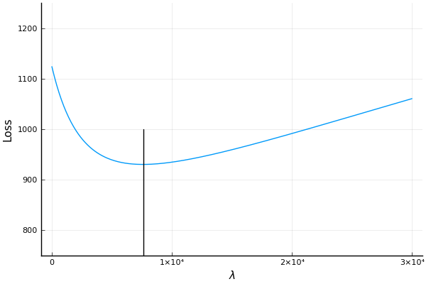
Searching for the best value using -fold cross validation.
Page built: 2021-03-04 using R version 4.0.3 (2020-10-10)