See the latest book content here.
6 Tricks of the Trade
A suggested reading for this chapter is Practical recommendations for gradient-based training of deep architectures.
A second epecific to Stochastic Gradient Descent Tricks
Another interesting reading which is to get an overview and light introduction to deep Learning is Deep Learning paper published in Nature.
6.1 Learning outcomes
- Considerations for choosing network architecture
- Hyper-parameter tuning methods and rules of thumb
- Optional: Gaussian processes for hyper-parameter selection
- Handling class imbalance and other data deficiencies
- Data augmentation
- Transfer learning
6.2 Hyper-parameter in Deep Learning
Hyper-parameters in Deep Learning are crucial for defining your model and to control the success of the training process of the defined model.
In general we can categorize the hyper-parameters into two groups:
Hyper-parameters for controlling the Optimization process: Optimizer hyper-parameters
Hyper-parameters for defining the model: Model Specific hyper-parameters
6.2.1 Optimizer hyper-parameters
These parameters are those related to the optimization process: Learning rate, Mini-Batch Size, Number of Epochs, weight decay, …
Learning rate. The calibration of the learning rate is quite crucial during the learning process. Indeed a too small value will require a very large number of epochs to converge while the algorithm might not converged by setting a too large value.
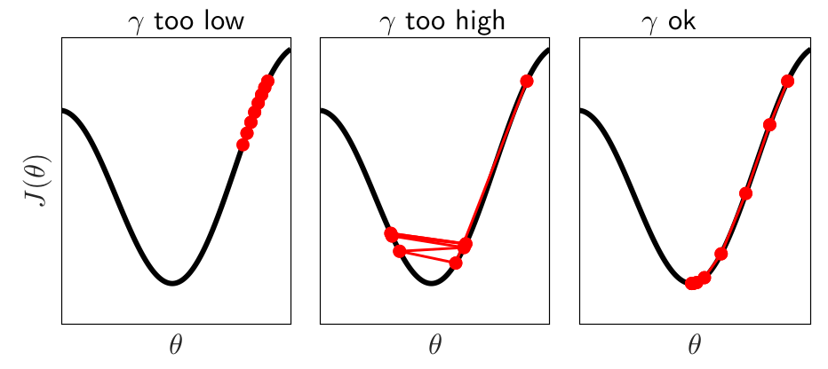
Figure 6.1: Effect of the learning rate setting
Moreover it is not recommended to use a constant learning rate. Indeed, even if a large value can help the algorithm to arrive quickly to a good solution, then it might oscillate around this state for a long time or diverge if the learning rate is maintained. A solution is to allow the learning rate to decay over time. In this framework the main procedures are:
exponential decay: αt=α0exp(−k×t)αt=α0exp(−k×t)
-
Inverse decay: αt=α01+k×tαt=α01+k×t
where α0α0 is the initial learning rate, kk controls the rate of the decay which will decrease at each epoch tt.
Another alternative is to reduce the learning rate by some factor every few epochs (also called Step decay). A common approach is to half the learning rate every 5 epochs, or by 0.1 every 20 epochs. A proposed heuristic is to track the validation error while training with a fixed learning rate, and if the validation error stops improving then reduce the learning rate by a constant (e.g. 0.5).
Mini-Batch Size. Remind that a Mini-Batch size of 1 sample corresponds to the stochastic training while a mini Batch size of the entire data is the batch training. A large size of the Mini-Batch can help the convergence process of the training algorithm but could be very expensive in term of memory and computation. A smaller Mini-Batch size which introduces more noise error and it is generally adopted for avoiding to be stuck in a local minima. A popular value of the mini batch size is 32. It is also well recommended to try subsequent values: 1, 2, 4, 8, 16, 32, 64, 128, 256.
Number of Epochs. The choice of the number of epochs is driven by the result of the Validation Error. We should train the model as many number of iterations as long as the validation errors keeps decreasing. The most common approach is to used the Early Stopping technique which consists to stop the training process when the validation error has not improved in the last 10 or 20 epochs.
Regularized tuning parameter. We have already see that the L2L2 regularization is the most exploited technique for preventing overfitting. This approach is also called as weight decay as this penalty introduced in the optimization algorithm encourages the weight parameters to decay toward zero. In statistics it is referred as shrinkage parameter because the penalty shrink the coefficient toward zero. The principle is to add a penalty term to the loss function on the training set in order to reduce the complexity of the learned model:
L(w,b)+λ2‖w‖2,L(w,b)+λ2∥w∥2, where λλ is called the weight regularization hyperparameter. Then at each iteration, the model will try to minimize the weights and the loss function. Thus it will keep the weight small and then preventing very large value of the weight and thus avoiding exploding gradient. Small values are generally tried first for controlling the contribution of each weight to the penalty.
But which values to use ?.
Heuristic from Goodfellow and colleagues (see Chapt 7 of Deep Learning Book)
``In the context of neural networks, it is sometimes desirable to use a separate penalty with a different coefficient for each layer of the network. Because it can be expensive to search for the correct value of multiple hyperparameters, it is still reasonable to use the same weight decay at all layers just to reduce the size of search space.’’
The weight decay is a key element during the training phase and the amoount of regularization is depending of each data set and architecture. Here some indications to consider for setting the weight decay hyperparameters:
It has been shown that weight decay is not like learning rates and the best value should remain constant throughout the training.
It might be worth to consider for this hyperparameter a grid search strategy if some difference due to the weight decay value is visible early in the training.
Possible classical choices: 10−310−3, 10−410−4, 10−510−5, and 0.
Experiments have also shown that smaller datasets and architectures seem to require larger values for weight decay while larger datasets and deeper architectures seem to require smaller values.
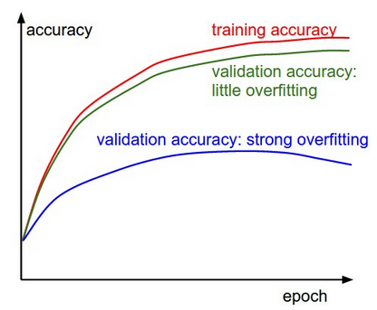
The following figures could indicate some direction to go. Let consider a classification task problem. In the figure below, the gap between the training and validation accuracy indicates the amount of overfitting. The blue validation error curve shows very small validation accuracy compared to the training accuracy and then indicates a strong overfitting. You should try to increase regularization as stronger L2 weight penalty or add some dropout strategy.
6.2.2 Model Hyperparameters
These parameters are related to the architecture of the network. Guideline for setting these parameters are not really clear. In the following, we collect some heursitics found from experiments.
Number of hidden units.. This parameter represents the capacity to learn and approximate any function. Only fewer number of hidden units might be sufficient for simple function. Then, more units are necessary for complex model. However, too many neurons might lead to overfit the dataset and limit to generalize to new sample.
First hidden layer. Experiments have shown better results by settig more neurons in the first hidden layer than than the number of inputs.
Number of layers. Increasing the number of layer for shallow network improves generally the performance (for example going to 2 hidden layers to 3). However, this improvement is very limited by going deeper (except for CNN).
Activation functions. There is no consortium of which activation functions to use. However, ReLu activation function is becoming the most used as is less computationally expensive than tanh and sigmoid. In the following some suggestions to start with:
For classification task, it is natural to use Sigmoid or Softmax activation function.
For regression task, a linear activation function is appropriate.
ReLU function is becoming more popular as the sigmoid and tanh functions might cause vanishing gradient problem.
However, ReLu function might cause dead neurons and the leaky ReLU function is then adopted.
Warning: ReLu function is only used in the hidden layers.
6.2.3 Some Heuristics
Some theoretical bounds of optimal topology are summarized in the following paper How many hidden layers and nodes? for two hidden layers model.
Heuristics 1: Simple first
“A popular heuristic is to incrementally build a more complex model. This means for example to try first a model with only one or two hidden layers and expand the network if the simple model fails.”
Heuristics 2: Increases number of neurons first
“A second heuristic is to increase first the number of hidden neurons before trying to increase the number of hidden layers when your model perform poorly. Indeed it is less computational expensive to doubling the size of a hidden layer than doubling the number of hidden layer.”
6.3 Hyper-parameters Optimisation procedures
The three main techniques for finding optimal values for the hyper-parameters are:
Grid Search
Random Search
Bayesian Optimisation
6.3.1 Grid Search
Grid Search is the most natural method for hyper-parameters tuning for Machine Learning models. The main idea is to test each possible combination of the hyper-parameters and select the one which give the best performance of your model. The performance is evaluated using k-cross-validation method. A grid is defined for indicating which values of the each hyperparameters are tested. However, this approach is generally not possible in Deep learning framework due to the computational burden issue. Indeed large neural network architecture require sometimes long time to train and so a grid search will take days/weeks and even months. Moreover, as the number of hyper-parameters increases, the cost of grid search increases exponentially.
Two ways for making Grid search faster:
Early stopping: the idea is to run all the grid points for one epoch, then discard the half that performed worse, then run for another epoch, discard half, and continue.
Embarrassingly parallel task: run all the different parameter settings independently on different servers in a cluster.
6.3.2 Random Search
Random Search is one variant of the grid search by randomly chosen points instead of points on a grid.
Bergstra and Bengio in Random Search for Hyper-Parameter Optimization mentioned that “randomly chosen trials are more efficient for hyper-parameter optimization than trials on a grid”
](images/gridsearch.jpeg) Figure 6.2: illustration from Random Search for Hyper-Parameter Optimization
Figure 6.2: illustration from Random Search for Hyper-Parameter Optimization
This strategy solves the curse of dimensionality as you do not need to increase the number of grid points exponentially. It is also possible to parallelized. However, it is not necessarily going to get anywhere near the optimal parameters in a finite sample.
6.3.3 Bayesian Optimisation
An alternative which is becoming widely used is the Bayesian Optimization techniques. The main idea of using a Bayesian approach is to pay attention to past results for exploring a better region.
The actual function f(θ)f(θ) we are trying to optimize (function of hyper-parameters) is really complicated.
Surrogate model
Bayesian Optimization defines a surrogate model (simple function) to approximate the objective function f(θ)f(θ). This surrogate model represents the prior belief about f(θ)f(θ).
After getting a certain number of points, the main idea is to condition on these to infer the posterior over the surrogate model using Bayesian regression modelling.
Gaussian Process (GP) is the most popular choice for defining the surrogate model. A Gaussian Process (GP) is a collection of random variables, where any finite number of these are jointly normally distributed.
GP is defined by the mean function m[θ]m[θ] and a covariance function (noted k[θ,θ′]).
We model our objective function f[θ]∼GP[m[θ],k[θ,θ′]]. A popular choice for the kernel function (covariance function) is an exponentiated quadratic kernel (with ℓ=1 and σ=1) will result in a smooth prior on functions sampled from the Gaussian process.
k[θ,θ′]=σ2exp[−12ℓ2(θ−θ′)T(θ−θ′)].
Thus, given some observations of f at t points f=[f[θ1],f[θ2],…,f[θt]] we desire to make prediction about the function value at a new point θ∗. The proprety of the GP tell us that This new function value f∗=f(θ∗) is jointly normally distributed with the observations f:
Pr([ff∗])=Norm[0,[K[θ,θ]K[θ,θ∗]K[θ∗,θ]K[θ∗,θ∗]]],
where K[θ,θ] is a t×t matrix where element (i,j) is given by k[θi,θj], K[θ,θ∗] is a t×1 vector where element i is given by k[θi,θ∗] and so on.
As an excercice you can determine the distribution of Pr(f∗|f) and so get the distribution of the function at any new point θ∗]
(Hint: use standard formula)
The following figure illustrates the GP by updating the mean and the uncertainty when data points are sequentially added.
](images/GP.png)
Figure 6.3: illustration from Gaussian process model
Acquisition function
The next key element is to define an acquisition function for choosing the next point to explore. This function tells us how promising a candidate it is.
The desire features of the acquisition function:
high for points we expect to be good
high for points we’re uncertain about
low for points we’ve already tried
Popular acquisition functions are:
Maximum Probability of Improvement (MPI)
Expected Improvement (EI)
Upper Confidence Bound (UCB)
Here we present the Expected Improvement (EI) which is the popular one:
EI(θ)=E[max{0,f(ˆθ)−f(θ)}], where f(ˆθ) is the current optimal set of hyper-parameters. It can be interpreted as: “if the new value is much better, we win by a lot; if it’s much worse, we haven’t lost anything”
There is an explicit formula for Expected Improvement (EI) under the Gaussian Process model.
EI(θ)={(μ(θ)−f(ˆθ)−ξ)Φ(Z)+σ(θ)ϕ(Z)if σ(θ)>00if σ(θ)=0 Z={μ(θ)−f(θ+)−ξσ(θ)if σ(θ)>00if σ(θ)=0 where μ(θ) and σ(θ) are the mean and the standard deviation of the GP posterior predictive at θ. Parameter ξ determines the amount of exploration during optimization and a recommended default value is 0.01.
The main steps of the algorithm:
For t=1,2,… repeat:
Find the next sampling point θt by optimizing the acquisition function over the GP: θt=argmaxθEI(θ|D1:t−1), where D1:t−1=(θ1,y1),…,(θt−1,yt−1)
Compute exact loss yt=f(θt) from the objective function f. We can also introduce some noise yt=f(θt)+ϵt
Add the sample to previous samples D1:t=D1:t−1,(θt,yt).
Update the GP.
Empirically Bayesian Optimization has been demonstrated to get better results using in fewer experiments, compared with grid search and random search.
You can explore this nice tutorial on Bayesian Optimization
6.4 Transfer Learning
Some key definitions of Transfer Learning concept and terminology
Transfer learning is the practice of reusing pre-trained models on a new task. It has been very popular in deep neural networks as it allows us to use deep neural architecture even if you have a small dataset.
Transfer learning exploits the knowledge of an already trained model on a new related problem (task).
Transfer learning can be viewed as an optimization process given rapid progress and improved performance for modeling the second task
Transfer learning is the process to transfer the weights that a network has learned at “task A” to a new “task B.”
Transfer learning it is not specific to deep learning (A Survey on Transfer Learning).
Transfer learning is becoming popular in computer vision and natural language processing (NLP) where Deep Neural Networks require a lot of data and a lot of computational power.
6.4.1 General Ideas
Transfer Learning is way to pick up a model “off the shelf” and to adapt it to your target task. You might take a model that has been already trained for one task (e.g., for classiying object) and then fine-tune it to accomplish another but relevant task.
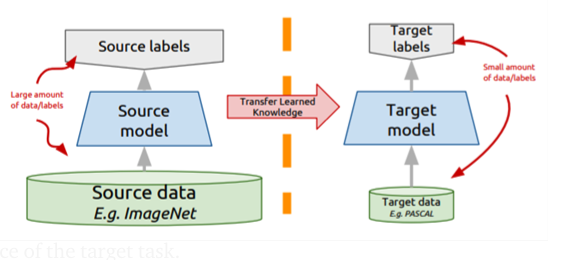 Figure 6.4: Main idea
Transfer Learning has been largely exploited in computer vision-related tasks as studies have have shown that features learned from very large image sets, such as the ImageNet, are highly transferable to a variety of image recognition tasks.
6.4.2 How to transfer knowledge from one model to another?.
Feature extrator. One way to achieve it is to chop off the top layer of the already trained model and replace it with a randomly initialized one. Then train the weight parameters only in the top layer for the new task, while all other weight parameters remain fixed (said frozen).
This approach is generally adopted when your data and the task are similar to the data and the task of the original pre-trained model. It is very relevant when you have a small data set to train your model for the target task. Moreover as you have fewer parameters to train you reduces the chance to have an overfitting issue.
![(Feature Extractors)[https://towardsdatascience.com/a-comprehensive-hands-on-guide-to-transfer-learning-with-real-world-applications-in-deep-learning-212bf3b2f27a]](images/TL_DS_DT.png) Figure 6.5: (Feature Extractors)[https://towardsdatascience.com/a-comprehensive-hands-on-guide-to-transfer-learning-with-real-world-applications-in-deep-learning-212bf3b2f27a]
Figure 6.5: (Feature Extractors)[https://towardsdatascience.com/a-comprehensive-hands-on-guide-to-transfer-learning-with-real-world-applications-in-deep-learning-212bf3b2f27a]
Fine-Tuning.
](images/finetune.svg) Figure 6.6: illustration of Fine-tuning concept
Figure 6.6: illustration of Fine-tuning concept
Fine tuning is a popular technique for transfer learning. The main idea is to exploit a “good” source model and then construct your target model by replicating all architecture and parameters from the source model, except the output layer. Then, all parameters are fine-tuned on the target dataset. Only the output layer of the target model needs to be trained from scratch meaning that you initialize the weights using a pre-trained model instead of initializing them randomly. It can be viewed as a warm start which will speed up the convergence. In this setting it is recommended to lower the learning rate in order to prevent changing the transferred parameters too early.
Fine-Tuning and/or Freeze
](images/freeze-fine-tune.png) Figure 6.7: illustration of Fine-tuning concept+ frozen
Figure 6.7: illustration of Fine-tuning concept+ frozen
We have seen that convolutional neural networks tend to learn edges, textures, and patterns in the first layers. The initial layers tend to capture generic features, while the later ones focus more on the specific task at hand. Moreover, features that detect edges, corners, shapes, textures, and different types of illuminants can be considered as generic feature extractors and be used in many different types of settings. However, the closer we get to the output, the more specific features the layers tend to learn, such as object parts and objects.
Then, you can decide to transfer all layers except the top layer or only transfer the first n layers. You might only freeze the first layer of the pre-trained model and fine tune the subsequent layers.
6.4.3 Unsupervised domain adaptation
Unsupervised Domain Adaptation is a learning framework to transfer knowledge learned from source domains with a large number of annotated training examples to target domains with unlabeled data only.
This transfer learning approach has been exposed by Yaroslav Ganin and Victor Lempitsky for Unsupervised Domain Adaptation by Backpropagation
The proposed architecture for unsupervised domain adaptation is represented in the following figure
](images/UDA-images.png)
Figure 6.8: illustration of source link
The proposed approach is based on three components:
Feature Extractor component is exploited. It will learn to perform the transformation on the source and target distribution
Label Classifier component will learn to perform classification on the transformed source distribution. Since, source domain is labelled
Label Domain Classifier component which is a neural network that will be predicting whether the output of the Feature Extractor is from is from source distribution or the target distribution.
The main idea is to exploit the Label Domain Classifier to get the model to be confused about the domain meaning to maximize this loss (by reversing the gradient). The key point is to confuse the Feature Extractor part in order it cannot create features that allow the domain classifier to work well but it still can create features that allow the label predictor to perform well (see more details in the original paper here)
6.4.4 Further Reading
- Chapter 11: Transfer Learning from Handbook of Research on Machine Learning Applications, 2009.
- How transferable are features in deep neural networks?
- Post on transfer learning
- A tutorial
- Notes from CS231 course
- Transfer Learning in Keras with Computer Vision Models
- Unsupervised Domain Adaptation by Backpropagation
6.4.5 Pre-trained Models
6.5 Data Augmentation
Data Augmentation is a popular technique in Deep Learning context to improve the performance of your model. Indeed, Deep Learning can accomplish complex tasks using deep networks which rely on a large number of parameters. However, to achieve a high accuracy the networks need a large amount of data and also a lot of diversity in the data to avoid overfit issues.
Data Augmentation can be a solution by applying different transformations on the available data to synthesize new data.
Data Augmentation can also address the class imbalance problem in classification tasks. For example in context of plain numerical data SMOTE technique The Synthetic Minority Over-sampling TEchnique is generally used.
6.5.1 Image Augmentation for Computer Vision Applications
Simple transformations to the image include:
geometric transformations such as Flipping, Rotation, Translation, Cropping, Scaling
color space transformations such as color casting, Varying brightness, and noise injection.
These simple transformations have been largely exploited and shown improvement of the model for computer vision tasks as image classification, object detection, and segmentation. However, these transformations are limited and might not be able to account all the possible variations.
An alternative is to use Deep Neural Network-based methods such as:
Adversarial Training
Generative Adversarial Networks (GAN)
Neural Style Transfer
See for more details the recent survey on Image Data Augmentation which illustrates how data augmentation can improve the performance of deep learning models.
6.5.2 Text Augmentation Techniques for Natural Language Processing
Easy Data Augmentation (EDA) for Natural Language Processing includes:
Synonym Replacement
Random Insertion
Random swap
Random deletion
However, such methods can struggle with preserving class labels.
Recently Wu et al. (2019) have proposed a conditional BERT (CBERT) model which extends BERT masked language modeling (MLM) task by considering class labels to predict the masked tokens.
Page built: 2021-03-04 using R version 4.0.3 (2020-10-10)